Nate Silver's Blog, page 165

Senate Update: Alaska, A Frontier For Bad Polling

The Senate race in Alaska is as important as any in the country. As we’ve described previously, Republicans can win a Senate majority by winning the race there along with those in five other deeply red states: Arkansas, Louisiana, Montana, South Dakota and West Virginia. But Alaska is probably the toughest “get” of the six for the GOP.

Unfortunately, Alaska has received very little polling — and just about every poll we do have from the state has been either an Internet poll, an automated poll or a partisan poll. The stronger pollsters seem to be avoiding the state — perhaps for good reason.

A new, partisan poll of Alaska came out over the weekend. The survey, conducted for Senate Majority PAC by Harstad Strategic Research, shows the Democratic incumbent Mark Begich leading his Republican opponent Dan Sullivan 45 percent to 40 percent. That contradicts the last two nonpartisan polls of the state, which had shown Sullivan ahead.

Senate Majority PAC’s goals are pretty clear; its mission is to “protect and expand the Democratic majority in the U.S. Senate.” Longtime readers will know that we’re not fans of partisan polls, which tend to be inaccurate and biased.

But defining a partisan poll can be tricky. Many pollsters release some polls on behalf of campaigns, while publishing other results under their own names. Some polls have ties to interest groups that aren’t well disclosed: For instance, the polling firm We Ask America is a subsidiary of the Illinois’ Manufacturers Association. Explicitly partisan blogs and websites have been commissioning more of their own polls in recent years (of course, many people would claim that traditional media outlets like Fox News and the New York Times have their own biases).

We’ve experimented a lot with different definitions of what constitutes a partisan poll over the years and decided we’re not inclined to play “poll police” in borderline cases. So since 2012, we’ve been excluding only polls conducted directly on behalf of campaigns or party groups like the Democratic Senatorial Campaign Committee and the Republican National Committee. Everything else gets included in the FiveThirtyEight model — including this weekend’s Alaska poll.

But the model has a defense mechanism: its house effects adjustment, which evaluates polls for signs of a partisan lean and adjusts them accordingly. In this case, the model detects a significant Democratic house effect in Harstad’s polls, and it treats the Alaska survey as showing the equivalent of a 1- or 2-percentage point lead for Begich, instead of a 5-point advantage. The poll still helps Begich some — his chances of winning the race jumped from 31 percent to 38 percent — but not nearly as much as if a nonpartisan pollster had shown the same result.

But there’s another reason to be suspicious of the poll — and others that purport to show Begich ahead in Alaska. As other commentators have noted, Alaska is a hard state to poll accurately. What we haven’t seen remarked upon is how those misses have come in one direction, almost always overestimating the performance of Democrats.

The table below lists Alaska results from our pollster ratings database, which covers polls conducted in the last three weeks of campaigns since 1998. (We’ll be publicly releasing this database soon.) For each race, I’ve compared the polling average against the actual margin, excluding the 2010 Senate campaign where the top two finishers were both Republicans, Joe Miller and Sen. Lisa Murkowski (who ran as a write-in candidate after losing her primary).

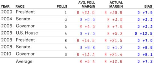
In every single race, the polls have shown a Democratic bias. In 2008, for instance, Begich was favored by almost 10 percentage points in the polls against the Republican incumbent Ted Stevens, but won by barely more than a percentage point. Also that year, the polls favored the Democrat Ethan Berkowitz to win the state’s at-large House district from the Republican incumbent Don Young, but Young prevailed instead. In 2004, the polls had the Democrat Tony Knowles, the state’s former governor, tied in his race against Murkowski, but Murkowski won by three points. In 2010, the Republican gubernatorial candidate Sean Parnell by a margin much larger than the polls anticipated. On average since 1998, polls of Alaska have had a 7-point bias toward Democrats.

The FiveThirtyEight model does not account for this property, but it’s something to keep in mind as you peruse polls of the state. The model does, however, include a “state fundamentals” estimate for each state, based on factors like fundraising and state partisanship, and includes it along with the polls.

The state fundamentals estimate does not receive very much weight in the model — it represents only about 15 percent of the projection in Alaska, for example, and as little as 5 percent in some other key states with more abundant polling.

Still, it can be interesting to look at. In Alaska, while our adjusted polling average puts Sullivan ahead by just one percentage point, the fundamentals estimate has him as an 8- or 9-point favorite instead. That gap of about seven points is right in line with the historical Democratic bias in Alaska polls.

Overall — also accounting for new polls in Louisiana and Georgia — the FiveThirtyEight forecast is not much changed. It shows Republicans with a 58 percent chance of winning the Senate majority, down just slightly from 59 percent on Friday.

NFL Owners May Be Overvaluing Goodell

NFL Commissioner Roger Goodell is under pressure to resign for his handling of Ray Rice, the former Baltimore Ravens running back who knocked out his then-fiancee in a casino elevator in March.

Rice was initially suspended for two games, in line with the NFL’s history of issuing shorter suspensions for domestic violence than for many other types of personal conduct violations — even though rates of domestic violence arrests are high among NFL players as compared with other crimes. Goodell announced changes to the league’s policy in August, introducing six-week suspensions for first-time domestic violence offenses and lifetime bans for repeat offenders. But the new policies were not applied retroactively to players like Rice.

Goodell came under renewed criticism this week after additional video of the casino incident was published by TMZ; it shows Janay Rice collapsing after the running back punched her. Ray Rice has since been released by the Ravens and suspended indefinitely by the NFL, but a number of reports have called into question Goodell’s claim that he had not seen the longer video at the time he decided on Rice’s initial two-game suspension.

Other reports imply that Goodell has the support of most of the league’s 32 franchises — in large part because of the NFL’s financial success. As Sports Illustrated’s Peter King wrote:

Goodell has so much goodwill in the bank in [the owners’] eyes that there’s no way—without definitive proof that the commissioner lied—they’d throw him, and his $44 million annual compensation, to the wolves. The goodwill includes a collective bargaining agreement with the players association through 2020 and lucrative TV contracts that pay each team about $150 million per year.

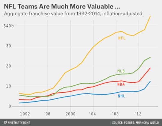
Indeed, the NFL is probably the most valuable sports league in the world. According to Forbes’s annual Business of Football valuations, its 32 franchises are worth a collective $45 billion. That’s nearly double that of Major League Baseball franchises, worth a collective $24 billion, and NBA franchises, worth $19 billion. (What about European soccer? The average NFL team is worth $1.4 billion dollars — more than all but four or five club teams in Europe.)

The NFL wasn’t always quite so dominant, especially relative to baseball. In 1991, when Financial World magazine issued valuations for the four major North American sports leagues (see Rodney Fort’s website for archived data), NFL franchises were worth an aggregate $6.5 billion (adjusted for inflation to 2014 dollars), not much more than the $5.5 billion for MLB teams. But NFL franchises have appreciated at an annual rate of 8.8 percent since then, compared to baseball’s 6.7 percent.

The bulk of that growth, however, occurred under Goodell’s predecessor, Paul Tagliabue. Since Goodell took over as commissioner in 2006, NFL franchises have risen in value by 32 percent, net of inflation, according to Forbes. That’s the lowest of the North American leagues by some margin. NHL franchises have increased in value by 114 percent, MLB franchises by 82 percent and NBA franchises by 65 percent over the same period (and Forbes is probably undervaluing the NBA, given recent franchise sale prices).

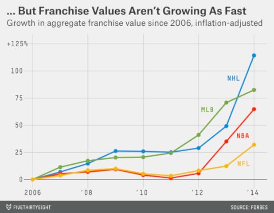
Broken down in terms of annual growth rates: NFL franchise values grew at an annualized rate of 11.7 percent from 1991 to 2006 under Tagliabue and just 3.5 percent per year since 2006 under Goodell.

The Forbes estimates aren’t perfect. All NFL franchises but the Green Bay Packers are privately held, and the league has very low rates of franchise turnover, with many teams having remained in the hands of the same family for decades. But the prices of recent franchise sales, like those of the Jacksonville Jaguars and Cleveland Browns, have closely matched the Forbes valuations.

The modest rate of franchise value growth under Goodell has come from a very high baseline — and perhaps some decline in the rate of growth was inevitable given how prodigiously they grew under Tagliabue. In absolute dollar terms — not percentages — NFL franchise values have risen by a collective $10.9 billion since 2006, compared with $11 billion for baseball, $7.5 billion for the NBA and $6.6 billion for the NHL. The NFL is still a hugely profitable business, and even poorly run franchises tend to make money because of the league’s aggressive revenue sharing and relatively favorable contractual agreements with players. According to Forbes, only the Detroit Lions lost money in 2013, and the league’s 32 franchises earned a collective $1.7 billion in operating income.

At the same time, the NFL did such a good job of expanding its reach and protecting its brand under Tagliabue and Pete Rozelle that even a mediocre commissioner could be in a position to look good. Compared to his predecessors and his counterparts in other leagues, Goodell’s value to the NFL’s bottom line hasn’t been quite so clear.

NFL Week 2 Elo Ratings And Playoff Odds

It’s a cliche: Every game counts in a league that plays just 16 of them. But Benjamin Morris’s findings in his debut Skeptical Football column were nevertheless striking: A Week 1 or Week 2 game can affect an NFL team’s chances of making the playoffs by as much as 20 or 30 percent.

We also see that reflected in FiveThirtyEight’s NFL Elo ratings playoff odds, a feature we debuted last week.

What are Elo ratings? The short version: Elo ratings are a simple mathematical system originally designed to rate chess players. They’ve since been adapted to a number of sports such as soccer, and we’ve adapted them to the NFL. The Elo ratings only account for fairly basic information like wins and losses, strength of schedule and margin of victory. There are more advanced systems out there, but Elo ratings are transparent, easy to calculate and we can do a lot of fun stuff with them, like simulating the rest of the season and calculating playoff odds. For more on the methodology, see here.

In our Week 1 ratings — which were based on a team’s Elo rating at the end of last season — the New England Patriots had a 73 percent chance of making the playoffs and the Miami Dolphins had just a 32 percent chance. But the Dolphins upset the Patriots, and now it’s almost even: New England is at 54 percent to make the playoffs and Miami at 50 percent.

Why such a big shift? Well, every game counts (especially a divisional game; our simulation accounts for playoff tiebreakers). But also, the Patriots now look slightly worse than Elo originally pegged them, and the Dolphins look slightly better. Before Week 1, Miami had projected to win 7.7 games; it now projects to win 9.1. In other words, one NFL win for the Dolphins was worth more than one win in the Elo standings because Miami’s Elo rating improved.

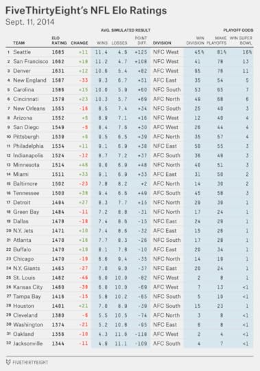
Here are the latest Elo ratings and playoff odds for all 32 teams:

A few other comments:

The teams with the largest gains on the week, in addition to the Dolphins, were the Minnesota Vikings, who gained 46 Elo points after demolishing the St. Louis Rams, and the Tennessee Titans, who added 38 Elo points after beating the Kansas City Chiefs. Both Minnesota and Tennessee are now better than even money to make the playoffs; the Titans are helped by playing in the league’s weakest division (although the NFC East might have something to say about that).It’s early, but perhaps we’re seeing the emergence of a Big Three. The Seattle Seahawks are the most likely team to win the Super Bowl, at 16 percent, followed by the San Francisco 49ers at 13 percent and the Denver Broncos at 11 percent. Then there’s a fairly big drop to the Carolina Panthers at 7 percent.Meanwhile, in the it’s-already-time-to-panic department, the Chiefs project to just a 6-10 record and have only a 13 percent chance of making the playoffs.

Elo ratings can also be used to derive point spreads. We strongly advise that you don’t bet on these, at least not without considering a lot of other information — Vegas betting lines are too sophisticated to be beaten by a simple system like Elo. Still, it’s fun to track their progress. Last week, they went 8-8 against point spreads as listed at Pro-Football-Reference.com.

There are some funky matchups this week. Elo has the Vikings at almost even money at home against New England, while Vegas has the Patriots as 3-point favorites. Another point of disagreement is Seattle at San Diego; Vegas has the Seahawks as 6-point favorites — a lot on the road against a playoff team. Elo thinks they should be favored over the Chargers by a field goal instead.

Registered Voter Polls Will (Usually) Overrate Democrats

Over the long run, Republicans and Democrats each win elections about half the time. This is not only a strong historical tendency1, but also one well predicted by political theory. A party that continually loses elections because it’s too far removed from the political center or because it appeals to too narrow a range of voters should seek to remedy that by expanding its coalition or moving toward the median voter — perhaps by compromising some of its ideological goals.

Sometimes the transition can be rough. The Republican Party, for example, is currently engaged in a battle between its more moderate and more conservative forces. It’s not clear the conflict between the Republican establishment and the so-called tea party is over. Nonetheless, parties usually become more moderate before long. In presidential elections, they’ve tended to nominate successively more moderate candidates the longer they’ve been out of the White House. Democrats, for instance, chose Bill Clinton in 1992 after losing with more liberal nominees in 1984 and 1988. And Republicans nominated more moderate candidates in Senate races this year than they did in 2010 or 2012.

But that the parties tend toward electoral parity doesn’t mean their coalitions are mirror images of each other. For a long time in American politics, Republicans have represented those voters who are in the majority (or plurality) demographically. A voter who is white, straight, suburban, Christian, middle-aged and middle income is quite likely to be a Republican. However, a voter who deviates from that profile in some respect — for instance, by being black, Hispanic, gay, Jewish, an atheist, young or by having completed an education beyond an undergraduate degree — is likely to be a Democrat. The majority of Americans deviates from that profile in at least one of those respects. That’s part of why a larger share of Americans have long identified as Democrats rather than Republicans.

Why would the GOP accept such an arrangement and take the smaller coalition? Doesn’t it defy the median voter theorem that I described before?

One reason may be that a less diverse coalition is easier to manage; Republican voters generally have more in common with one another than Democratic voters do. A straight, single Latina mother living close to the poverty line in El Paso, Texas, is very likely to be a Democrat. So is a white, wealthy, PhD recipient with a same-sex partner in Madison, Wisconsin. But the straight Latina voter and the gay white voter may have few interests in common.

The other consolation to the GOP is that the Americans affiliated with the Republican Party are more likely to turn out to vote, especially in midterm elections. Whites turn out at greater rates than racial minorities; older Americans at greater rates than younger ones; wealthier ones at greater rates than poorer ones. To editorialize for a minute, I think voting ought to be made easier — you ought to be able to vote in a box, with a fox, in your house with the click of a mouse, or in any other way that damn well pleases you. But in the status quo, demographic groups differ in their ease of access to voting and their overall level of political engagement — and those Americans who tend to have easier access and higher levels of engagement are more likely to vote Republican.

That was a long windup, so here’s the pitch: Polls of so-called likely voters are almost always more favorable to Republicans than those that survey the broader sample of all registered voters or all American adults. Likely voter polls also tend to provide more reliable predictions of election results, especially in midterm years. Whereas polls of all registered voters or all adults usually overstate the performance of Democratic candidates, polls of likely voters have had almost no long-term bias.2

This represents one difference between FiveThirtyEight’s Senate projections and several other forecast models. Our program “translates” registered voter polls to make them equivalent to likely voter results. With some exceptions, other forecast models do not. This is one reason the FiveThirtyEight model tends to show a more favorable outcome for Republicans.

And history is on our side. I compared likely voter polls conducted during the final three weeks of Senate campaigns since 1990 against the actual results in each state.3 I looked for evidence of statistical bias in these polls — for example, a poll that put the Republican ahead by 2 percentage points in Arizona when the Republican won by 9 points. That poll would have had a 7-point Democratic bias. The table below reflects the average statistical bias of likely voter Senate polls in each election since 1990, broken down between midterm and presidential years.

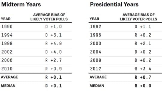
As the table shows, the bias has varied quite a lot from year to year. In 1998, the average likely voter poll overstated the performance of the Republican candidate by almost 5 percentage points. But there was an opposite and nearly equal bias in the next midterm in 2002, when the polls overstated the performance of Democrats by about 4 points. (To drop a bomb in the #nerdwar, results like these ought to make one very skeptical of models that implicitly or explicitly assume the error in polls is uncorrelated from state to state or from survey to survey. At least as often when the polls miss they miss in the same direction; that contributes to the uncertainty of the forecast and makes an “unexpectedly” good showing by one party or the other more likely.)

But while likely voter polls may show a bias toward one party in any given election, they’ve been fair over the long run. In the average midterm year since 1990, Senate likely voter polls have had a bias of 0.1 percentage points toward the Republican candidate — that is to say, virtually no bias. In presidential years, they’ve had a 0.7-point GOP bias. That’s very small compared with the overall error in Senate polls and probably reflects statistical noise rather than anything systemic.

What about registered voter polls? We can infer that, because likely voter polls have no long-term bias and registered voter polls show more favorable results for Democrats, registered voter polls usually have a Democratic bias.

We’ve kept diligent records on registered voter polls for the past couple of election cycles. In 2010, the average likely voter poll was 6 percentage points more favorable to the Republican than the average registered voter poll of the same state, reflecting a historically large turnout/”enthusiasm gap.” Although likely voter polls had a slight Republican bias that year — about 1 percentage point — registered voter polls had a 5-point Democratic bias.

Our data on registered voter polls before 2010 is scattered. During the final several weeks of a campaign, pollsters usually release likely voter results exclusively. Or if they do publish registered voter numbers, it is as a complement to their likely voter results. The registered voter results receive less emphasis from the news media and are sometimes not preserved in polling databases.

However, we can come up with a reasonable proxy for registered voter surveys by comparing the partisan affiliation of voters in each year’s national exit poll against the affiliation of a larger sample of American adults. In particular, for years before 2010, I’ve compared the party affiliation numbers in the exit poll against those among all adults in polls conducted by the Pew Research Center, Gallup and CBS News/The New York Times.

This evidence suggests that the turnout gap almost always favors Republicans. In 2008, for instance, Democrats had a 7-point partisan ID advantage in the national exit poll. That’s impressive, but it’s smaller than the 9- or 10-point advantage Democrats had throughout the year in polls of all adults. Overall, since 1990, there has been a 2.7 percentage-point turnout gap favoring Republicans in midterm years, and a 1.9-point gap favoring them in presidential election years, we estimate.

Because polls of likely voters are nearly unbiased, that implies polls of registered voters would usually have a Democratic bias. For example, in 2008, we estimate that polls of registered voters would have a 2.5 percentage-point Democratic bias, while polls of likely voters had almost zero partisan bias on average.

There are some years when the registered voter polls would have been more accurate. In 2012, for example, the average likely voter poll understated the performance of Democratic candidate by more than 3 percentage points; registered voter polls would have provided a more accurate picture. But for each year like 2012, there are more like 2002 or 1994, when even the likely voter polls had a Democratic bias and where registered voter polls would have made the problem worse. In 1994, for example, likely voter polls already overrated the standing of Democrats by 3 percentage points; registered voter polls would have had closer to a 5-point Democratic bias instead.

We estimate that on average in midterm years since 1990, registered voter polls have had a 2.6 percentage-point Democratic bias — compared against likely voter polls, which have been unbiased.

The data in presidential election years is somewhat more equivocal. On average, registered voter polls of Senate races have had a 1.1 percentage-point Democratic bias in these years, we estimate, whereas likely voter polls have had a 0.7-point Republican bias. A lot of that was caused by 2012, when the polls had a substantial Republican bias. Looking at medians rather than averages produces similar results to midterm years: Likely voter polls have been unbiased, whereas registered voter polls have had a median Democratic bias of 2 percentage points.

That’s why our model adjusts registered voter polls in the way it does; their Democratic bias is fairly predictable, especially in midterm years.

And there’s another reason to adjust registered voter polls to a likely voter basis. As the election gets closer, a higher and higher proportion of pollsters will release likely voter results exclusively or in conjunction with registered voter results. A model that’s ambivalent about the distinction might misinterpret the switch between registered and likely voter numbers as reflecting “movement” toward the Republican Party.

Tennis Has A Big Three-And-A-Half

We wrote Monday that the Big Four of men’s tennis — Roger Federer, Rafael Nadal, Novak Djokovic and Andy Murray — dominate the sport despite the seemingly seismic upsets at the U.S. Open on Saturday. Kei Nishikori and Marin Cilic upset Djokovic and Federer, respectively, in semifinals and will play the final Monday. But Djokovic, Nadal and Federer remain far ahead of those two upstarts and other younger challengers in the rankings.

Murray, though, is a different story. He hasn’t reached a final in 14 months. He’ll fall out of the Top 10 if Cilic wins Monday.

Murray has always been a bit of a different story — an awkward fit in the Big Four. It’s often seemed like a Big Three and Murray. The other three each have at least seven Grand Slam titles and have been ranked No. 1 for more than 100 weeks each. Murray has two Grand Slam titles and peaked at No. 2.

Murray’s overall record at the biggest tournaments makes him mostly worthy of his Big Four status, but it also establishes how far behind the other members he is. Despite repeatedly and unfortunately having to face them, Murray trails only those three players in career success, among anyone whose Grand Slam career began in the past quarter-century.

We compiled annual results for 19 players at the four Grand Slams and the nine Masters tournaments, the 13 events where nearly all the top players compete, pulling data from Tennis Abstract. Then we calculated the number of ranking points each player earned at those tournaments — using the current point distributions — and divided by the maximum number of points each could have earned. So, for example, to earn 100 percent of possible points, a player would have to sweep all 13 tournaments. We prorated this year’s numbers and split the 800 additional points Monday’s winner will earn between Cilic and Nishikori.

Our 19 players are the Big Four, the second line of five players mentioned in the companion article — Cilic, Nishikori, Grigor Dimitrov, Ernests Gulbis and Milos Raonic — and their contemporary Juan Martin del Potro, and the nine non-Big Four male players who reached the No. 1 ranking and started playing Grand Slam tournaments in 1990 or later (1990 is when the Masters events began, under a different name): Lleyton Hewitt, Andy Roddick, Gustavo Kuerten, Marat Safin, Juan Carlos Ferrero, Yevgeny Kafelnikov, Carlos Moya, Marcelo Rios and Patrick Rafter.

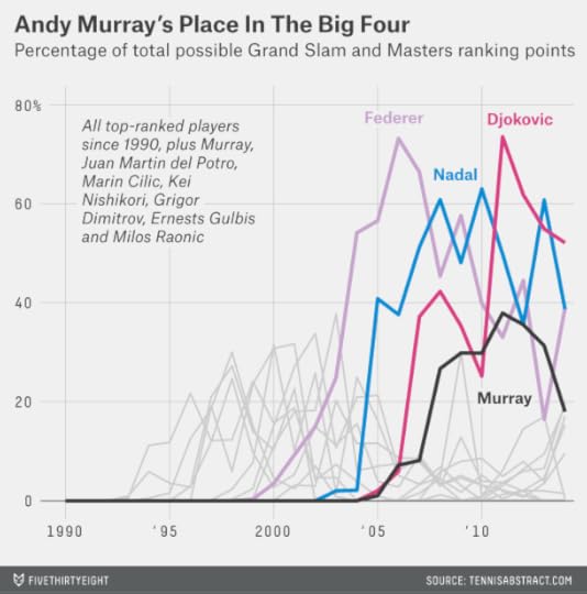
What’s striking about Murray is how much his curve is dwarfed by those of Federer, Nadal and Djokovic — and yet how much his curve towers over almost everyone else’s. His peak season, in 2011, is better than the best season of each of the non-Big Four players we studied. Even Murray’s fifth-best season, in 2010, is better than the best season of four former top-ranked players: Roddick, Moya, Rafter and Kafelnikov. Or, if “better” isn’t appropriate for a season that doesn’t include a Grand Slam title, then Murray’s season in which he had the fifth-highest weighted average level at big tournaments was more consistently good than the career best years for four players who reached the No. 1 ranking.

We concluded our earlier piece by saying the second line and del Potro should aspire to match Murray. That’s no small achievement — and it could be big enough to reach the No. 1 ranking he’ll probably never attain, because these younger players are less likely to have to contend with the likes of Federer and Nadal for the entirety of their careers.

It’s Not The End Of An Era For Men’s Tennis

The reigning oligarchs of men’s tennis — Roger Federer, Rafael Nadal, Novak Djokovic and Andy Murray — have devolved a smidgen of power to the sport’s second line.

For six years, the Big Four have ruled the sport, hoarding its biggest titles and topping the rankings. This year, five younger men have broken through, most dramatically on Saturday at the U.S. Open. First Kei Nishikori stunned world No. 1 Djokovic in four sets. Then Marin Cilic straight-setted five-time Open champ Federer. Nishikori and Cilic will play in Monday’s final, the first Grand Slam final for each man and the first without a member of the Big Four since 2005.

Federer lightly applauded his younger rivals’ modest achievements in his post-match press conference Saturday. After congratulating Cilic for his great play, Federer called it “definitely refreshing to some extent” to have new names in a Grand Slam final, and added, “I hope they can play a good final.”

Federer pointed out that any tennis writers who downgraded the Big Four’s stock when Stan Wawrinka won in Australia in January had to explain the finals of this year’s French Open and Wimbledon, which featured exclusively himself, Nadal and Djokovic. “But this is another chance for you guys, you know,” Federer told the room full of journalists. “So you should write what you want. I don’t think so, but … .”

Federer is both right and wrong. The Big Four really have been slipping. That can be hard to spot because each player has had a complicated arc over the last few seasons. Djokovic gained, lost and regained the No. 1 ranking, with Nadal and Federer each holding it for a spell. Federer has rebounded swiftly from a mediocre 2013. Murray has dropped fast after winning two Grand Slam titles and an Olympic gold medal over a 12-month run that ended last summer.

Group the four together, though, and the decline is more apparent. In 2011, they won an absurd 84 percent of their maximum possible total of ranking points at the 13 annual tournaments that bring together the world’s best male players: the Masters and Grand Slam events. That share has fallen steadily each year since, to 66 percent so far this year. Some regression to the mean was inevitable, but the Big Four’s grip on the sport has fallen below the mean, to its lowest level since 2006, according to data compiled from the stats site Tennis Abstract.1

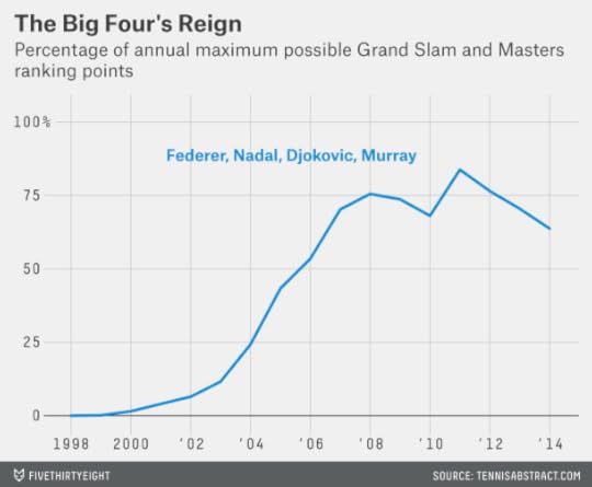
That still leaves the Big Four in a much stronger state than the prior ruling class ever reached.2

The five younger upstarts — Cilic and Nishikori, plus Grigor Dimitrov, Ernests Gulbis and Milos Raonic, who are between age 23 and 26 and reached their first Slam semis this year — have mostly been defined by their arrested tennis development. They’ve shed the previously apt Lost Boys title with career years this season. But they’re more of a Medium Five or Next Five than a Fab Five, though at least, unlike that Michigan quintet, one of these five will win a major title in a Monday championship.

There wasn’t an obvious name for the group until Cilic perfectly described it after his near-perfect match Saturday. In his press conference, Cilic referred three times to the sport’s “second line.”

“The guys there are from second line, are moving closer and they are more often at the later stage of the tournament,” Cilic said. “They are going to get only better; they’re not going to get worse.”

Cilic was including Australian Open champ Wawrinka in his list, but Wawrinka, 29, is older than three of the Big Four. For our purposes, we’re not going to include him so that the “second line” is a separate generation from the current stars, who are between ages 27 and 33.

There is one major name missing from the second line’s roster: Juan Martin del Potro, who turns 26 this month. He and the second line are the six youngest men ranked in the Top 20. Even Monday’s champion probably won’t finish this year with a season as good as del Potro’s best. In 2009, the year he turned 21, del Potro won the U.S. Open, came within a set of the French Open final and reached the quarterfinals of six Masters tournaments.

Injuries have kept him from maintaining that level, and from playing any tennis for the last six months. But already del Potro has achieved in his career more than the quintet of his peers will have achieved after Monday’s final: one major title; three Masters finals (the other five have two total); and seven titles at the 500 level, the next tier down from Masters events (the other five have five, and three of those belong to Nishikori). Before Monday, del Potro was the only man who is now under 27 and had played in a Grand Slam final. Federer had won 12 Grand Slam titles before turning 27.

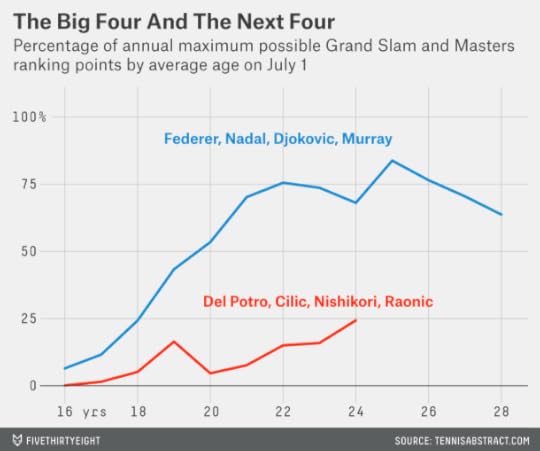
Adjusting for age shows how much the second line lags the first, even in a career year. The most accomplished four of the bunch — del Potro, Cilic, Raonic and Nishikori — have won 24 percent of their maximum possible total of ranking points at the Masters and Grand Slam events this season. The Big Four, at roughly the same average age in 2010, won 68 percent. At age 20, the Big Four won 53 percent to the second line’s 5 percent at the same age. And this year, all of the Big Four could finish ahead of all five of the second line in the rankings.

So the second line isn’t the generation we need to take over men’s tennis. But it’s the one we have — at least until the generation of Wimbledon quarterfinalist Nick Kyrgios and other promising teenagers launches its challenge. And the second line is playing its best tennis this season. Heading into the U.S. Open, Dimitrov, Nishikori and Raonic all were on pace for career highs in dominance ratio (DR), the ratio of returning points win percentage to opponent returning points win percentage — a good marker of overall level. And Cilic and Gulbis were serving better than ever, with career highs in ace percentage and first-serve win percentage.

Through the lens of the past week, Nishikori looks like the most impressive member of the second line. He beat three top-five seeds in his last three matches at the Open. But his DR was below 1 in his last two wins, meaning he won them with little margin.

Cilic, by contrast, straight-setted two top-six seeds in his last two matches, and was forced into just one tiebreaker. He has also been more durable than Nishikori has during their careers. The two youngest members of the group, Dimitrov and Raonic, have stayed mostly healthy, too, and have climbed the most steadily and quickly.

One of those three or del Potro probably will finish with the best career of the second line’s generation. Whoever does will be hard pressed even to match the achievements of Murray. He’s by far the weakest member of the Big Four, an oligarchy that remains dominant even in its decline.

Polls Show Path Of Least Resistance To GOP Majority

Pollsters are picking up the pace after a slow start in this midterm election season. Sunday featured the release of a trio of NBC News/Marist polls of the Senate races in Arkansas, Kentucky and Colorado, while the online polling firm YouGov released polls of almost every Senate race in conjunction with the New York Times and CBS News.

The bottom line is not much has changed. The FiveThirtyEight forecast model gives Republicans a 65.1 percent chance of winning the Senate with the new polling added, similar to the 63.5 percent chance that our previous forecast gave them on Friday.

But the path to a Republican majority is becoming a little clearer — and the problem for Democrats is that it runs through six deeply red states.

Republicans have long been favored to win back the seats in Montana, West Virginia and South Dakota, three states where Democratic incumbents have retired. Montana and West Virginia are virtual locks for Republicans. South Dakota is slightly less certain only because of the presence of a third-party candidate, the former Republican Senator Larry Pressler. However, Pressler was at only 6 percent of the vote in the YouGov poll, lower than in other recent surveys.

The GOP’s next two easiest targets are in Louisiana and Arkansas, where the Democratic incumbents Mary Landrieu and Mark Pryor are struggling with electorates that have turned much redder since their tenure in office began.

Both the NBC/Marist and YouGov polls put Pryor behind among likely voters in Arkansas. Each poll also showed Pryor in a tie with his challenger, Republican Rep. Tom Cotton, among registered voters, but that’s not entirely good for news for Democrats; several earlier polls of the state had shown Pryor ahead among registered voters, leaving open the prospect that he could win the election with a strong turnout. Pryor retains a chance to keep his seat — about a 30 percent chance, according to our forecast — but he may need both a strong turnout and a strong close to his campaign.

The new polling did not affect our forecast in Louisiana, since the YouGov poll was a survey of the state’s Nov. 4 open primary and not its probable Dec. 6 runoff between the top two candidates, Landrieu and the Republican Bill Cassidy. (The FiveThirtyEight forecast is projecting the runoff results in Louisiana and not the primary; it appears unlikely that either Landrieu or Cassidy will get 50 percent of the vote on Nov. 4, which would avert the runoff.) The poll was nevertheless bad news for Landrieu, since it showed her with just 36 percent of the vote against 48 percent for the top two Republicans, Cassidy and Rob Maness, combined. Based on previous runoff polling, Republicans have about a 70 percent chance of winning the seat, about the same as in Arkansas.

The sixth red state, which could be decisive in giving Republicans a majority, is Alaska. There, the YouGov poll gave the Republican Dan Sullivan a 6-point lead over the Democratic incumbent Mark Begich, reversing a July YouGov poll that had put Begich 12 points ahead.

It could be easy to make too much of the YouGov poll. It had a small sample size — about 400 likely voters — in a notoriously hard-to-poll state. Nonetheless, it’s among the only recent polls of Alaska and shows a result more in line with how other red-state Democratic incumbents like Pryor and Landrieu are polling.

The FiveThirtyEight model evaluates a series of “fundamentals” factors in each state in addition to the polling. Ordinarily, these receive relatively little weight in the model, but they get more in states like Alaska where the polling is thin. In Alaska, the fundamentals model puts Begich 8 points behind Sullivan, principally because his left-of-center politics are further removed from Alaska’s median voter than Sullivan’s and because Begich only narrowly won his election in 2008. Public fundraising is another factor in the fundamentals estimate; Sullivan has raised nearly as much in individual contributions as Begich, in contrast to other states where Republican challengers face larger fundraising gaps against Democratic incumbents.

Because of this, the FiveThirtyEight model already had Begich as a slight underdog before the new poll was released — although he’s a heavier underdog now, with a 30 percent chance of keeping his seat, similar to Landrieu and Pryor.

But we shouldn’t lose sight of the big picture. Republicans can win the Senate solely by winning Alaska, Arkansas, Louisiana, Montana, South Dakota and West Virginia, states which voted for Mitt Romney over Barack Obama by an average of 19 percentage points in 2012.

Another potentially vulnerable Democratic incumbent got some better news. In Colorado, both the NBC/Marist and YouGov polls put the Democratic incumbent Mark Udall ahead of his Republican challenger, Rep. Cory Gardner — as did a Rasmussen Reports poll conducted late last week. Udall is now a 63 percent favorite in Colorado, improved from a very slight underdog when the FiveThirtyEight model launched last week.

However, if Begich holds on in Alaska or Pryor does in Arkansas, Republicans retain some backup options. Iowa and North Carolina are tossups, according to the FiveThirtyEight model. Democrats remain favored in Michigan — this weekend’s YouGov poll put the Republican Terri Lynn Land slightly ahead, but the consensus of surveys show Democrat Gary Peters with the lead — but it remains a highly competitive race. Republicans face longer odds in New Hampshire and Minnesota, but they aren’t entirely safe for Democrats either.

Democrats could greatly complicate Republicans’ math by picking off one or more Republican-held seats. Kentucky, which once appeared to be Democrats’ best option, may be fading as an alternative. The NBC/Marist and YouGov polls were the latest in a long string of polls to show Republican minority leader Mitch McConnell ahead of the Democratic challenger Alison Lundergan Grimes; McConnell’s chances of keeping his seat are now up to 84 percent, according to the FiveThirtyEight forecast. The Democrats have slightly better prospects in Georgia and Kansas, although the latter state remains exceptionally difficult to forecast after the Democratic candidate, Chad Taylor, ended his campaign last week. (YouGov polled Kansas but it did not include the center-left independent candidate Greg Orman in its survey, who could caucus with Democrats if he wins.)

A mild piece of good news for the Democrats is that the turnout gap may not be as large as it was in 2010. Both YouGov and NBC/Marist released results among both registered voters and likely voters in each of the states they polled — and on average, their likely-voter models showed the Republican candidate doing a net of about 2.5 percentage points better than in the registered-voter version of their surveys. That’s in line with the historical average gap between registered and likely voters in midterm years — rather than the 6-point gap that persisted throughout 2010.

The FiveThirtyEight model automatically shifts registered-voter surveys toward Republicans to make them equivalent to likely-voter polls; this is one of the reasons our forecast is slightly more favorable to Republicans than others you might encounter. It’s likely that other models will show a shift toward Republicans and come to more closely match ours as more polling firms begin to release likely voter results.

Introducing NFL Elo Ratings

If you followed FiveThirtyEight’s coverage during the World Cup, you know that we’re big fans of the World Football Elo Ratings. They’re based on a relatively simple system developed by the physicist Arpad Elo to rate chess players. But they can be adapted fairly easily for other head-to-head competitions from baseball to backgammon.

We thought we’d have a little fun and extend them to American football. In an accompanying post, you’ll find our initial Elo ratings for all 32 NFL teams (at this point, the ratings are based on a team’s standing at the end of last season, discounted slightly to reflect reversion to the mean). We’ve also developed a simulator program that plays out the NFL schedule thousands of times and projects a team’s likelihood of making the playoffs, based on a team’s record up to that point in time, its Elo rating, its remaining schedule and the NFL’s various tiebreaker rules. We plan to update these projections at the end of every week.

But first (inspired somewhat by The New York Times’s personification of its election model, Leo), we thought we’d “interview” the Elo system about how it does its work.

FiveThirtyEight: What are some of some of your best qualities?

Elo: I’m simple, transparent and easy to work with. I can do a lot with a little, such as calculating point spreads and the probability of either team winning a game.

Can I use you to beat Vegas?

I wouldn’t try that. Vegas lines account for a much wider array of information than I do. When Nate backtested me, he found that I got 51 percent of games right against the point spread. That’s not nearly enough to cover the house’s cut, much less to make a living.

We noticed that you have the Seattle Seahawks favored by 10 points in their Thursday-night game against the Green Bay Packers, while Vegas has the Seahawks as six-point favorites instead.

That’s a perfect example. Has anything strange been going on with the Packers?

Well, their star quarterback, Aaron Rodgers, was injured. Now he’s back!

If this Mr. Rodgers fellow is as good as you say he is, that could account for the difference. I don’t know anything about him. I only keep track of the final scores, the dates of games and where the games were played.

So what good are you?

Think of me as a benchmark. I do a pretty good job of accounting for the basic stuff — wins and losses, margin of victory, strength of schedule. I also retain a memory from past seasons, so I know that the Jacksonville Jaguars aren’t as likely to win the Super Bowl as the Denver Broncos. Can we get to some more technical questions?

Um … what are your parameters?

That’s more like it. Like K, for instance; K is my favorite parameter.

What makes K so special?

Elo: K tells me how much to update my ratings after each game. In a sport like baseball, where there are lots of games, any one additional game doesn’t tell you all that much, so K takes on a low value. In the NFL, it’s much higher. Specifically, it’s the number 20. That may not mean anything to you, but if you set K a lot higher than that, I’d be a nervous wreck and bounce around too much from game to game. And if you made K much lower, I’d be hopelessly sluggish and too slow to notice changes in the quality of team’s play.

I noticed the Detroit Lions have an Elo rating of 1467. What does that mean?

Elo: An average team has an Elo rating of 1500 — so your Lions are not so hot. But it could be a lot worse. In 2009, the Lions got all the way down to a rating of 1223. Most NFL teams wind up in the range of 1300 to 1700.

We’re still not quite sure how your ratings work. If you have one team at a 1650 and another at 1400, what does that mean?

If it makes things easier, you can translate my ratings into a point spread. Take the difference in my ratings and divide by 25. It’s that simple.

So, if one team is rated 250 Elo points higher than the other, that works out to a spread of 10 football points.

Precisely.

What about home-field advantage?

I can account for that, too. Historically, it’s been worth about 65 Elo ratings points or 2.6 NFL points. Just add that to the point spread.

What if you want to calculate a team’s probability of winning?

That’s pretty easy, too, although you’ll need a formula for it. In a game between Team A and Team B, Team A’s win probability is equal to:

Pr(A) = 1 / (10^(-ELODIFF/400) + 1)

Where ELODIFF is Team A’s Elo rating minus Team B’s Elo rating.

Let’s say Team A wins. Its Elo rating will improve?

Yes. One of my more appealing properties is that a team’s Elo rating will always improve after it wins and always decline after it loses. How much it improves will depend on how much of a favorite or an underdog it was.

So, like after the 2008 Super Bowl …

I can predict where you’re going with that question. I’ll admit that I didn’t have the New York Giants rated so highly compared to the New England Patriots. But the Giants’ Elo rating improved a lot after they won that game — more than the Patriots’ would have if they’d won instead. I may have my flaws, but unlike a lot of you human beings, I know how to fix them. The lower a team is rated, the easier for it to gain ground by proving me wrong.

Do you also account for margin of victory?

Affirmative. I took some inspiration from the soccer ratings, which account for goal differential in addition to the game result. But this is one of the more complicated parts.

For the NFL, I start by adding one point to team’s margin of victory and then take its natural logarithm. Then I multiply that result by the K value. That means I’m more moved by big wins than narrow ones, although there are diminishing returns. I’m not so impressed by the fifth touchdown when a team is ahead 28-0.

That seems simple enough.

It would be, but that isn’t all there is to it. We haven’t talked about my autocorrelation problem. It’s a little embarrassing.

Go on. “Autocorrelation”? Was that the weird David Cronenberg movie ?

Autocorrelation is the tendency of a time series to be correlated with its past and future values. Let me put this into football terms. Imagine I have the Dallas Cowboys rated at 1550 before a game against the Philadelphia Eagles. Their rating will go up if they win and go down if they lose. But it should be 1550 after the game, on average. That’s important, because it means that I’ve accounted for all the information you’ve given me efficiently. If I expected the Cowboys’ rating to rise to 1575 on average after the game, I should have rated them more highly to begin with.

It’s true that if I have the Cowboys favored against the Eagles, they should win more often than they lose. But the way I was originally designed, I can compensate by subtracting more points for a loss than I give them for a win. Everything balances out rather elegantly.

The problem comes when I also seek to account for margin of victory. Not only do favorites win more often, but when they do win, they tend to win by a larger margin. Since I give more credit for larger wins, this means that their ratings tend to get inflated over time.

Is this also a flaw with the soccer Elo ratings?

Possibly. You may want to reconsider what you wrote about Germany.

So, how do you correct for this?

It isn’t complicated in principle. You just have to discount the margin of victory more when favorites win and increase it when underdogs win. The formula for it is as follows:

Margin of Victory Multiplier = LN(ABS(PD)+1) * (2.2/((ELOW-ELOL)*.001+2.2))

Where PD is the point differential in the game, ELOW is the winning team’s Elo Rating before the game, and ELOL is the losing team’s Elo Rating before the game.

It’s a little ugly, but we all have our vices.

I see that you have ratings for this year’s teams, but they haven’t played any games yet! How does that work?

I take their rating from the end of last season and discount it slightly. Specifically, I revert it to the mean by one-third. Remember that the mean Elo rating is 1500. So, if a team finished last season with a rating of 1800, I’ll revert it to 1700 when the new season begins. This whole notion of “season” is strange to me, by the way. We don’t have them in chess.

For now, the ratings are all about which teams were good last year?

Technically speaking, a game affects my ratings forever once it’s played, just with a smaller and smaller weight that gradually diminishes to almost nothing over time. But, yes, for the time being, my ratings are mostly about who was good last season. Games toward the end of the season will count more, especially games during last year’s playoffs.

Thanks for taking the time! So, you’re saying we should take the Seahawks?

How about a nice game of chess?

See the Week 1 Elo ratings and playoff odds.

NFL Week 1 Elo Ratings

Each week throughout the NFL season, we’ll be publishing Elo ratings for teams and using them to simulate the remainder of the season, and calculate each team’s chances of making the playoffs and winning the Super Bowl. Read about our methodology for details about how the system works.

Elo ratings have been applied in many endeavors, from soccer to chess; we’ve simply taken the system and revised it to work with NFL data. Elo ratings have many virtues, including being simple and transparent. However, they’re based on a very limited set of information — only the final scores of games and home-field advantage is accounted for. Therefore, we very much doubt that they can consistently beat Las Vegas betting lines; the point spreads and win probabilities listed here are purely for fun and will not reflect important factors such as key injuries or personnel changes.

The two charts below show the initial 2014 NFL Elo ratings, which are based on a mean-reverted version of ratings from the end of the 2013 season, as well as the league’s Week 1 matchups.

Upheaval In The Kansas Senate Race Is Making Our Chart Kinky

If you’ve revisited our Senate forecast landing page, you may have noticed something a little different. The probability distribution showing how many Senate seats the Republicans might end up with is no longer a nice bell-shape-type curve. Instead, it has a kink.

What’s going on here? Why are Republicans more likely to end up with 50 or 52 seats than 51?

The reason has to do with the independent candidate in Kansas, Greg Orman, and which party he’s said he’ll caucus with should he win his election against the Republican incumbent, Pat Roberts. An Orman victory looks like a much more realistic prospect now that the Democratic candidate, Chad Taylor, has ended his campaign (although the Kansas secretary of state said Taylor cannot formally remove his name from the ballot). This is an extremely difficult race to forecast, but pending further information, our model gives Orman about a 45 percent chance of winning.

Orman has said that “if one party is clearly in the majority,” he will “seek to caucus with the party that was in the majority as that would be in the best interest for the state of Kansas.” In other words, his decision is contingent on how the other Senate races go.

We’re interpreting Orman’s statement to mean the following:

If after this year’s elections are complete, Democrats control at least 50 seats without Kansas (but counting the independents Bernie Sanders of Vermont and Angus King of Maine, who already caucus with them), Orman will caucus with Democrats.But if Republicans control at least 51 seats without Kansas, Orman will caucus with them instead.

The kink in the graph is the result of Orman potentially giving a party a “bonus” senator should it reach a majority without him. For example, if Republicans finish at 50 seats without Kansas, Orman might not join them. But at 51, he would, which would bring them up to 52.

What about that instance where Republicans are stuck on exactly 50 seats without Orman, while Democrats are at 49? In that case, Orman’s decision would determine Senate control. If he joined the Democrats, the Senate would be split 50-50 and Democrats would represent the majority party because of the tiebreaking vote of Vice President Joe Biden. If he joined the Republicans, they’d control the Senate 51-49.

Our assumption is that there’s a 75 percent chance Orman will caucus with the Democrats should that situation arise. This is similar to the assumption we made for King two years ago. Like King, Orman rates as left of center by the various ideology measures we track. His stated policy positions are similar to those of a moderate, red-state Democrat; he’s said he believes “in Second Amendment rights of Americans to keep and bear arms,” but he also advocates an amnesty program for undocumented immigrants and supports abortion rights. Orman was formerly a member of the Democratic Party, having run briefly for Senate as a Democrat in 2008.