Menzie David Chinn's Blog, page 9

Identities, Parameters and Regressions

A reader comments:

Your final jab in this post regresses the state output gap on the fiscal gap. You then conclude that there is a positive relation between the two and that this somehow implies that a reduction in gov’t spending is a drag on the economy. I’ll just point out that …. that gov’t spending is a component of GSP. Of course they’re positively related.

I think this comment reflects a commonplace confusion between identities, functional relationships, and reduced form coefficients.

For instance, consider that at the industry level for a state, such as in data reported by BEA here, total private (agriculture, mining, through manufacturing through other services) and government has to sum to total gross state product (in current lexicon state GDP). So, one would think that regressing total output on government output has to yield a positive coefficient. Run the regression over the 2005Q1-15Q3 period (the entire available sample) for Wisconsin:

GDPWI,t = 18829.71 – 0.215GOVWI,t + ut

Adj-R2 = -0.02. Bold denotes significance at 10% msl using HAC robust standard errors.

Lest you think this proves higher government spending causes less output, well, consider the same regression for Kansas.

GDPKS,t = 262893.4 + 5.895GOVKS,t + ut

Adj-R2 = 0.34. Bold denotes significance at 10% msl using HAC robust standard errors.

This is a lesson I learned as an undergraduate — do not appeal to an accounting identity for information about a coefficient.

Let’s turn to an example that is more familiar. We all know the expenditure side definition of GDP from macro:

Y ≡ C + I + G + EX – IM

I stress in my undergraduate courses that one cannot use identities to explain how the world works, or more concretely, when G changes, how does Y. For that, one needs a model.

So, the hapless regression-runner might regress Y on G, asserting one must get a positive coefficient since G is by construction a component of Y. But in fact different theories yield different implied coefficients.

Suppose aggregate supply is given by Y = Yn = ΦF(K,N), and aggregate demand is given by Y = fn(G, T, M/P), where K, N are given. Then the correlation between Y and G is … zero!

Suppose P is predetermined within a period, and aggregate demand takes the same form as above. Then the correlation between Y and G is positive, but not necessarily one (it’ll depend on the marginal propensity to consume, interest sensitivity of investment, interest sensitivity of money demand, etc.).

Suppose P depends positively on the output gap (i.e., a Phillips Curve holds), such that P = Pe + θ(Y-Yn). Then the correlation is positive, but (holding all else constant) smaller than that in the previous example.

Suppose P depends positively on the output gap, and the fiscal authorities rely on a “fiscal rule” that achieves counter-cyclical stabilization, e.g., G = φ(Y-Yn), φ < 0. Then the implied correlation between Y and G is now negative.

One could in principle estimate the reduced form coefficient in the first three cases (after accounting for omitted variables, etc.); the parameters (e.g., θ) would require determining an appropriate instrumental variable. The correlation can always be calculated; whether it’s meaningful is another question.

Bottom Line: Identities do not tell you about behavior. Inferring causality is hard, but if one wants to tell a story, one has to try to deal with the data in an intelligent way.

Another weak quarter for U.S. GDP

The Bureau of Economic Analysis announced today that U.S. real GDP grew at a 0.5% annual rate in the first quarter. That’s disappointing, even by standards of the weak growth that has become the norm since getting out of the Great Recession.

Real GDP growth at an annual rate, 1947:Q2-2016:Q1, with historical average (3.1%) in blue and post-Great-Recession average (2.1%) in red.

Housing investment was one bright point. Another was growth in government spending at the state and local level which more than made up for a drop at the federal level. An important drag came from the decline in exports, reflecting economic weakness outside the United States. The biggest negative was a drop in nonresidential fixed investment, which by itself subtracted 3/4 of a percent from the Q1 annual growth rate.

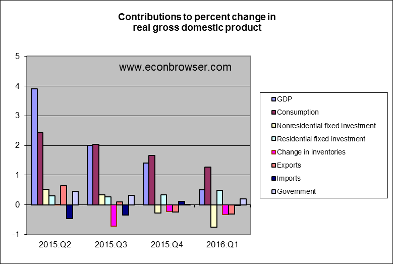
Further declines in investment spending in the oil-producing sector contributed to that. Domestic spending on mining exploration, shafts, and wells is now down more than $100 billion at an annual rate (about 6/10 of a percent of total U.S. GDP) from the levels seen in the summer of 2014.

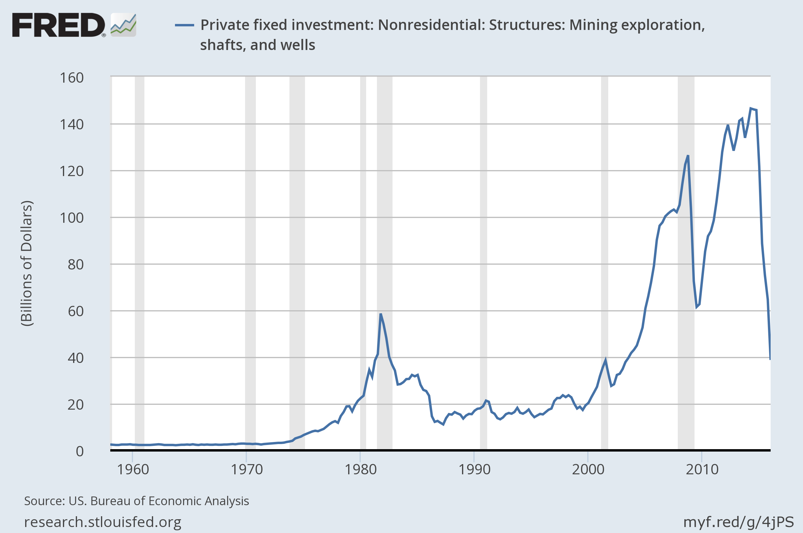
Expenditures on private fixed nonresidential structures investment in mining exploration, shafts, and wells. Source: FRED.

The disappointing Q1 GDP numbers brought our Econbrowser Recession Indicator Index up to 15.7%. The index uses today’s data release to form a picture of where the economy stood as of the end of 2015:Q4. That’s still significantly below the 67% threshold at which our algorithm would declare that the U.S. had entered a new recession.

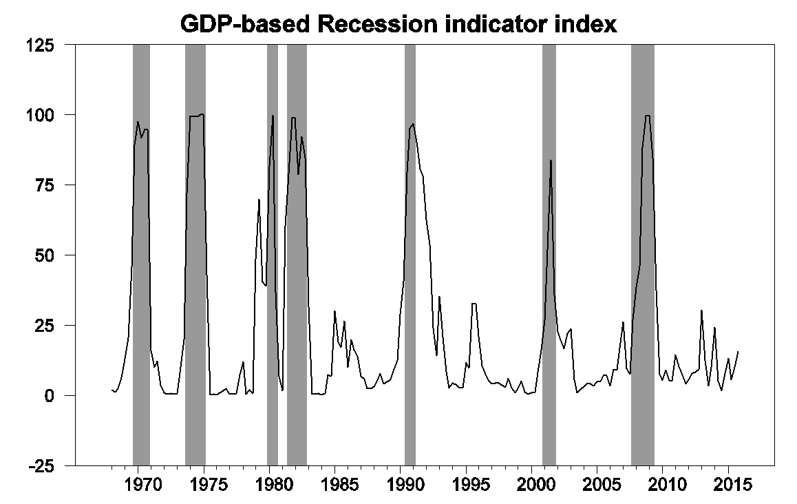
GDP-based recession indicator index. The plotted value for each date is based solely on information as it would have been publicly available and reported as of one quarter after the indicated date, with 2015:Q4 the last date shown on the graph. Shaded regions represent the NBER’s dates for recessions, which dates were not used in any way in constructing the index, and which were sometimes not reported until two years after the date.

U.S. growth is certainly facing some significant headwinds, and lower oil prices do not appear to have helped. Nevertheless, the employment numbers have been showing strong momentum, and housing can make further positive contributions in the coming two years. Maybe not enough to get us back to 3%. But we can still hope to get back to 2%.

Two Employment Goals: Kansas, Wisconsin

In Governor Brownback’s re-election campaign, he committed to 25,000 new jobs per year in his next term. This is reminiscent of Governor Walker’s August 2013 promise to create 250,000 new private sector jobs over the four years of his first term, by January 2015. How are things going?

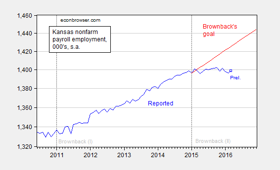
Figure 1: Kansas nonfarm payroll employment (blue), and Governor Brownback’s goal, assuming linear growth. Log scale. Source: BLS and author’s calculations.

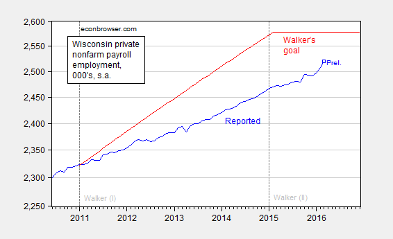
Figure 2: Wisconsin private nonfarm payroll employment (blue), and Governor Brownback’s goal, assuming linear growth. Log scale. Source: BLS and author’s calculations.

Since net employment growth in Kansas is essentially zero, Kansas is short by 26.7 thousand relative to trend. Despite the fact that I’ve allowed for extra time for Governor Walker’s promise, Wisconsin remains 58.1 thousand short.

For more on Kansas, see [1] and [2]. For more on Wisconsin, see [3].

Kansas: “This other Eden, demi(Austrian)-paradise”

On reading my recent post on Kansas economic performance in the reign of Brownback, which included this graph:

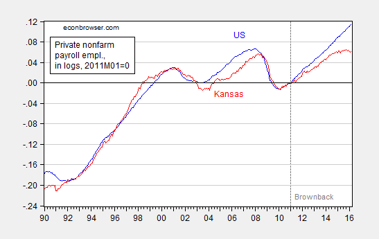
Figure 1: Private nonfarm payroll employment in Kansas (red), in US (blue), in logs normalized to 2011M01=0. Dashed line at 2011M01, Brownback term begins. Source: BLS, author’s calculations.

A&M Professor/Extension Economist Levi Russell writes “Your analysis is highly flawed”.

He then refers me to a post a year ago, critiquing both Paul Krugman’s post “This Age of Derp, Kansas Edition”, as well as my post.

Below the childish title of Paul Krugman’s latest post is a simplistic analysis of the state of the Kansas economy. Krugman references another post by Menzie Chinn that is slightly more sophisticated. I’ll focus on Krugman’s post but will refer to Chinn’s post as well.

…

Since Chinn and Krugman both mention California, let’s have a look at this “boom” in California. For whatever reason (he doesn’t say why he chooses these states), Chinn plots a business indicator from the Philly Fed for California, the US as a whole, Minnesota, Wisconsin, and Kansas. The graph clearly shows faster growth for CA, MN, and the US as a whole than for WI and KS. This is supposed to be a result of fiscal policy and evidence that KS and WI governments (with Scott Walker as its governor) are wrong for implementing right-wing policies.

…

That doesn’t imply, as Krugman states, that we should abandon our skepticism of the effectiveness of gov’t intervention. As I’ve shown here, a more nuanced analysis doesn’t tell the same neat little story about the Wheat State as those told by Krugman and Chinn.

Let me preface my comments by noting it is an honor to be lumped in with Paul Krugman.

One might excuse Professor Russell for not knowing how bad things would get over the year following his post, but in fact he has doubled down on his view that fiscal policy does not explain the evolution of the Kansas economy. In February, he wrote:

… the constant drumbeat from the [Kansas Center for Economic Growth] that the Kansas economy is weak due to the Brownback tax cuts is rather silly. Kansas has had strong private employment growth when compared with neighboring states since the tax cuts have gone into effect. As the recent “Rich States, Poor States” report indicates, two of Kansas’ biggest industries, oil and aircraft, have been under significant stress recently. This is, of course, not caused by the recent tax policy change in Kansas. Agriculture can certainly be added to that list.

Time to look at the data.

First, one cannot appeal to weather, cattle prices, wheat prices, oil prices, or even the aircraft industry’s woes, to explain the Kansas disaster. Consider the following out of sample forecasting exercise. I first estimate an error correction model with Kansas and US GDP over the 2005Q2-2010Q4 period:

(1)   ΔyKSt = -8.49 – 0.38yKSt-1 + 0.78 yUSt-1 + 1.46ΔyUSt-1 + 0.002droughtt + ut

Adj-R2 = 0.60, SER = 0.0085, N = 23, DW = 1.77, Breusch-Godfrey Serial Correlation LM Test = 2.07 [p-value = 0.16]. Bold face denotes statistical significance at 10% msl, using HAC robust standard errors. y denotes log real GDP, and drought is the Palmer Drought Severity Index for Kansas (PDSI, lower is more severe).

The data used in this analysis (and for calculations in Figures 3 and 4) are here. Log Kansas and US GDP appear I(1) (fail to reject Elliott-Rothenberg-Stock unit root test) and Kansas PDSI (borderline) rejects a unit root.

Using this ECM to dynamically forecast out of sample in an ex post historical simulation (i.e., using realized values of US and Kansas GDP, and the drought variable), I find that (1) actual Kansas GDP is far below predicted (5.3 billion Ch.2009$ SAAR, or 3.9%, as of 2015Q3), and (2) the difference is statistically significant. This is shown in Figure 2.

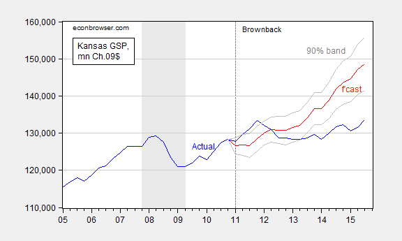
Figure 2: Kansas GDP, in millions Ch.2009$ SAAR (blue), ex post historical simulation (red), 90% band (gray lines). Forecast uses equation (1). NBER defined recession dates shaded gray. Source: BEA, NBER, and author’s calculations.

Note that historical simulation incorporates the effect of drought, despite the fact that the coefficient enters with significance only at the 21% level. In other words, based on historical correlations of Kansas GDP with national, and weather, Kansas should have performed measurably better.

Now, the last refuge the defenders of the Kansas experiment is to say it’s the agricultural or oil sectors, and/or it’s the aircraft industry’s woes, or maybe the plotting of the Illuminati. In Professor Russell’s critique of a Kansas Center for Economic Growth (KCEG) analysis, he uses all three (but omitting the role of the Illuminati).

As the recent “Rich States, Poor States” report indicates, two of Kansas’ biggest industries, oil and aircraft, have been under significant stress recently. This is, of course, not caused by the recent tax policy change in Kansas. Agriculture can certainly be added to that list.

My view: Whenever someone quotes Rich States, Poor States as if it were a source of reliable analysis, watch out!! But let’s take at face value this assertion – it’s anything but fiscal policy.

Let me systematically appraise each of these alternative explanations.

First, re-estimate equation (1) over the entire 2005Q1-2015Q3 period. The drought variable (the Kansas PDSI) does not enter with statistical significance at even the 50% msl. So maybe drought is it, but it doesn’t show up statistically.

Second, substitute in for the PDSI either the real wheat price (CPI deflated), real oil price (core CPI deflated) or the real cattle price (CPI deflated) for the drought variable, and once again the respective coefficients are not significant at the 50% msl, or for cattle is significant at the 50% msl, but with the wrong sign. (Note: log real wheat and cattle prices appear I(1), so I enter in first differences, while PDSI and log real oil prices appear I(0), so I enter in levels).

Hence, one is quickly exhausting the set of possible excuses for the Kansas dropoff.

What about aircraft production? I’ve addressed this in a previous post (Professor Russell shares certain views with Ironman in this regard), but why not repeat? Figure 3 shows a decomposition of growth on a quarter-on-quarter basis (not annualized).

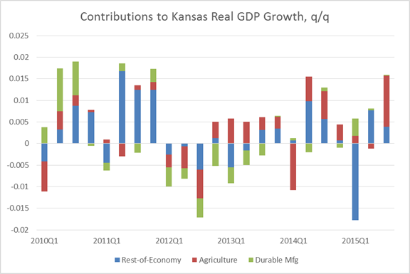
Figure 3: Contributions to real GDP growth, from agriculture (red), durable manufacturing (green), and rest-of-economy (blue). Source: BEA and author’s calculations.

At certain junctures, durable manufacturing and agriculture do subtract from growth; at other times add. But it has been quite some time since these factors have exerted a drag on output growth. Consequently, recent lagging performance cannot be attributed to the factors that Professor Levi highlights.

Finally, what about fiscal policy? Figure 4 shows the correlation between two variables: the gap between actual and predicted Kansas GDP, and the gap between the actual government spending on goods and services and trend (from 2005-2010). Well, as expected, the bigger the shortfall in government spending, the bigger the shortfall in growth.

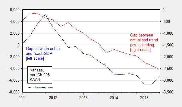
Figure 4: Gap between actual and predicted Kansas GDP (blue), and gap between actual and trend Kansas government spending on goods and services (red), both in millions in Ch.2009$ SAAR. Predicted GDP is from ex post historical simulation using equation (1). Trend government spending is exponential trend over 2005-2010 period. Source: BEA and author’s calculations.

The positive correlation is statistically significant. A regression yields the following result:

(2)   Δy_gapt = 5.76 + 2.39Δg_gapt-1 + ut

Adj-R2 = 0.09, SER = 1193.7, N = 18, DW = 0.94. Bold face denotes statistical significance at 10% msl, using HAC robust standard errors. y_gap denotes gap between actual and predicted Kansas GDP, g_gap denotes gap between actual and 2005-2010 exponential trend in Kansas government spending on goods and services.

The slope coefficient is statistically significant at the 6% msl. The confidence interval would encompass the conventional regional multiplier of approximately 1.5 [1]. What’s omitted is tax revenues –- revenues are now down about 2% relative to 2008Q1 peak [0]. That would have exerted an expansionary effect, but since I’ve also omitted transfers, it’s hard to say what the bias would be on the point estimate.

I conclude with my standard graph of GDP growth of the ALEC darlings and betes noire, Kansas and Wisconsin, and Minnesota and California, respectively, because Professor Russell could not discern the basis for my choice of states.

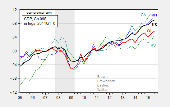
Figure 5: Log Gross State Product for Minnesota (blue), Wisconsin (bold red), Kansas (green), California (teal) and US (black), all normalized to 2011Q1, seasonally adjusted at annual rates, in Chained 2009$. Source: BEA, and author’s calculations.

Notice that pre-recession Kansas was growing faster than the other states and the nation; in the era of Brownback, well, the graph says it all, if you didn’t believe the econometrics.

Digression on fixed effects: At least back in June 2015, Professor Russell made a point of highlighting the difference in extent of slack in the Californian economy vs. the Kansas, arguing that when there is lots of slack, employment growth will tend to be fast. Hence, in his view, the relatively slow Kansas employment growth in Figure 1 is due to the smaller amount of slack, as measured by unemployment. However, apparently, Professor Russell has forgotten about fixed effects. Over the 1976-2007 period, California unemployment is typically about 0.77 percentage points higher than the national average; so the March 2016 California rate of 5.4% is only 0.4 percentage points higher than the national average. By that criterion, California’s labor market is tight. The Kansas situation is the opposite. On average, Kansas unemployment is 1.67 percentage points lower than the national average, and yet, as of March, it is only 1.1 percentage points lower. Hence, there would seem to be more ecnomic slack in Kansas than in California, by this criterion. Given this, the argument that California employment growth is faster because of more slack seems dubious to me. (Additional graphs of CA vs. KS in employment and coincident indices here).

Causes and consequences of the oil price decline of 2014-2015

At the NBER Annual Conference on Macroeconomics in Cambridge last week I participated with Steven Kamin of the Federal Reserve Board and Steven Strongin of Goldman Sachs in a discussion on commodity prices. You can watch a video of our discussion at the NBER web site.

Charles Wyplosz on the Eurozone Crises

“A Crisis that Should Not Have Happened”

Spring is the time of events at the University of Wisconsin-Madison. On Monday, among the other conferences and talks, the Jean Monnet European Union Centre of Excellence, the Center for European Studies, and the Department for Political Science hosted a fascinating (and at times provocative) discussion by Professor Charles Wyplosz of the Graduate Institute-Geneva.

The subtitle to this post is the title for the first slide of his presentation (the entire presentation is here):

A debt crisis

Collapse of the interbank market

Politically-charged bailouts

Ever widening conditionality

Intense summitry

ECB under threat

He characterizes all these as “institutional failures”. Much of the terrain he covered is familiar to those who have followed the eurozone crisis: while the the eurozone member countries had accumulated large debts by 2009, that wasn’t the entire story; fiscal discipline was never achieved pre-crisis; there was no lender of last resort; the absence of a unitary banking union was fatal; and so forth.

The entire presentation is here, but I’ll focus on a few key points. First, high level summitry was completely ineffective; this point was illustrated by all the summits (vertical lines) and the course of sovereign spreads, in the figure below.

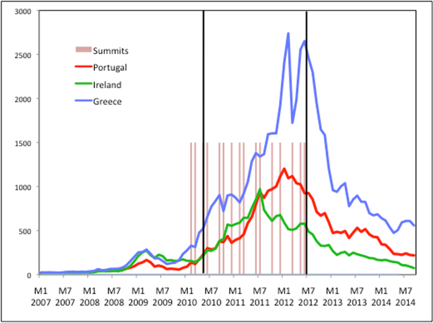
Source: Wyplosz (2016).

Spreads only come down with the ECB’s Draghi committing to “whatever it takes”.

Another point, the ECB was (way) behind the curve in responding to the crisis.

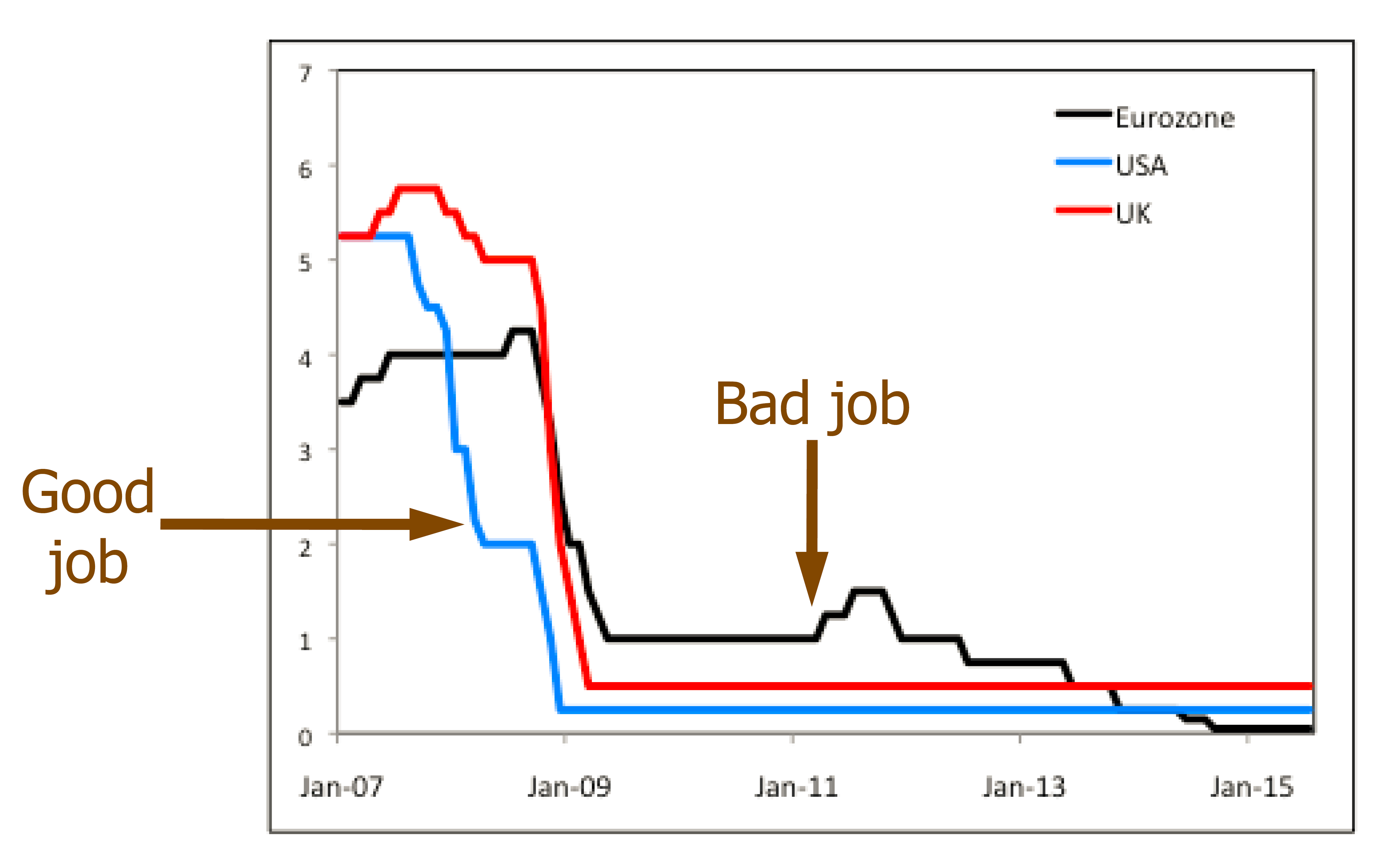
Source: Wyplosz (2016).

Not only was the ECB slow to cut rates, it actually raised rates prematurely.

One rather interesting point Wyplosz makes is that fiscal discipline is necessary, discipline of the sort American states have. This discipline would be implemented by way of a cyclically adjusted budget balance requirements.

While the cyclically adjusted balance is a better metric than a unadjusted balance, it’s not clear to me that such an arrangement would be sufficient to underpin a monetary union, given the absence of a eurozone-wide government that can effect substantial transfers, as does the Federal government in the US (via marginal tax rates, unemployment insurance, etc.) (my views on this subject laid out here).

Wyplosz’s arguments are laid out more comprehensively and formally here. And a way forward on restructuring the outstanding (and usnsustainable) levels of public debt in the eurozone member countries is laid out here.

“Kansas loses patience with Gov. Brownback’s tax cuts”

The experiment continues…

From CBS News today:

Brownback took office on a pledge to make Kansas friendlier to business and successfully sought to cut the top personal income tax rate by 29 percent and exempt more than 330,000 farmers and business owners from income taxes. The moves were popular in a Legislature where the GOP holds three-quarters of the seats.

The governor argued that Kansas had to attract more businesses after a “lost decade” in the early 2000s, when private sector employment declined more than 4 percent.

The predicted job growth from business expansions hasn’t happened, leaving the state persistently short of money. Since November, tax collections have fallen about $81 million, or 1.9 percent below the current forecast’s predictions.

Not only is predicted job growth missing, currently employment is below prior peak. It’s hard to argue for long term diverging trends as the explanation, given the long run co-trending of national and Kansas employment. In that context, the recent (since 2011M01) dropoff is remarkable.

Figure 1: Private nonfarm payroll employment in Kansas (red), in US (blue), in logs normalized to 2011M01=0. Dashed line at 2011M01, Brownback term begins. Source: BLS, author’s calculations.

The article continues:

“We’re growing weary,” said Senate President Susan Wagle, a conservative Republican from Wichita. While GOP legislators still support low income taxes, “we’d prefer to see some real solutions coming from the governor’s office,” she said.

So even after two more ruinous years, the whistling continues, just with fewer die-hards.

For further context, here’s a graph depicting economic performance of some ALEC-darlings (Wisconsin, Kansas ranked at 9 and 27 respectively) and ALEC betes noire (Minnesota, California ranked at 45 and 46).

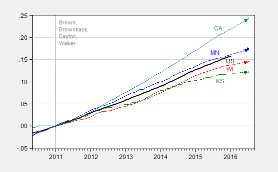
Figure 2: Coincident indices for Minnesota (blue), Wisconsin (red), Kansas (green), California (teal) and US (black), and implied levels from leading indices, all normalized to 2011M01=0. Source: Philadelphia Fed, January 2016 releases, and author’s calculations.

Thinking about The Great Leap Forward

When Technocrats Are Pushed Aside

Nearly 56 years ago, with the beginning of the second Five-Year Plan, Chairman Mao called for a “Great Leap Forward”. The objective was rapid development of the agricultural and industrial sectors in such a way as to catch quickly with both the Soviet Union and eventually the West. A focus was on use of mobilization by political means of large amounts of labor in order to circumvent the need for imported inputs including machinery.

Political mobilization as a means of achieving goals that are otherwise assessed as unrealistic by technocrats is noteworthy. In particular, key aspects of the Great Leap Forward included:



Abolishment of private property and moving agricultural production into state owned communes.

A goal of doubling steel production, in part by way of backyard furnaces.

Massive investment in infrastructure, primarily irrigation projects.

I’ll focus on the doubling of steel production as an example of failure to think through how to properly implement a program can lead to enormous waste. From Kung and Lin (EDCC, 2003):

… significant proportions of [the rural labor force] were being diverted to activities totally unrelated to agriculture, most notably the smelting of iron and mining and transporting ore in the so-called backyard furnaces. As was the case with water conservancy works, these projects similarly required that the highly fragmented and localized interests be unified. Moreover, as these were primarily industrial projects and their effective execution required managerial skills and expertise that were rarely available in the smaller collectives, the larger commune arguably provided the organizational context within which a faster pace of rural-based industrialization could be made possible.

However, the economic costs of this diversion were colossal. First, the 3 million tons of steel produced in these backyard furnaces was of such poor quality that at least half of it was considered wasted. Second, unintentionally many commune authorities were so preoccupied with iron and steel manufacturing in the autumn of 1958 that they neglected to harvest the crops, which were simply left to rot in the fields. This diversion of resources is estimated to account for 28.6% of the overall grain output collapse, a factor that was secondary only in importance to excessive procurement, according to one estimate.

Fixed investment rose; and so initially did grain and steel production.

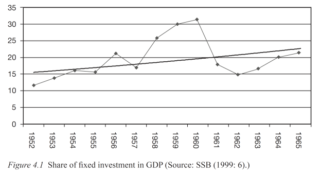
Source: Bramall (2009)

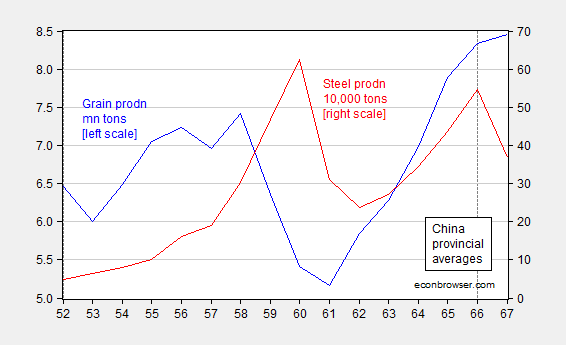
Figure 1: Average of provincial production of grain, in millions of tons (blue), and of steel, in 10,000 tons (red). Source:

What happened in the wake of essentially un-analyzed attempt to drastically re-orient the Chinese economy? Agricultural and industrial output collapsed. The ensuing famine resulted in 30-45 million deaths.

A ideologically driven committed “big push” involving lots of resources, unguided by careful analysis of how policies will be implemented, and likely effects, will almost certainly result in waste of monumental proportions and other unintended consequences.

More on the Great Leap Forward here and here, and Chinese development here.

A financial hockey stick

Yesterday I was at the 31st annual NBER conference on macroeconomics (along with fellow blogger Mark Thoma). Among the many interesting contributions was development of an extended data set on 25 different indicators for 17 advanced economies going back to 1870 by Jorda, Schularick and Taylor (2016).

The authors described one of their findings as a “financial hockey stick”. After nearly a century of stability, loans by banks to the nonfinancial sector began after 1950 to grow systematically faster than GDP around the world.

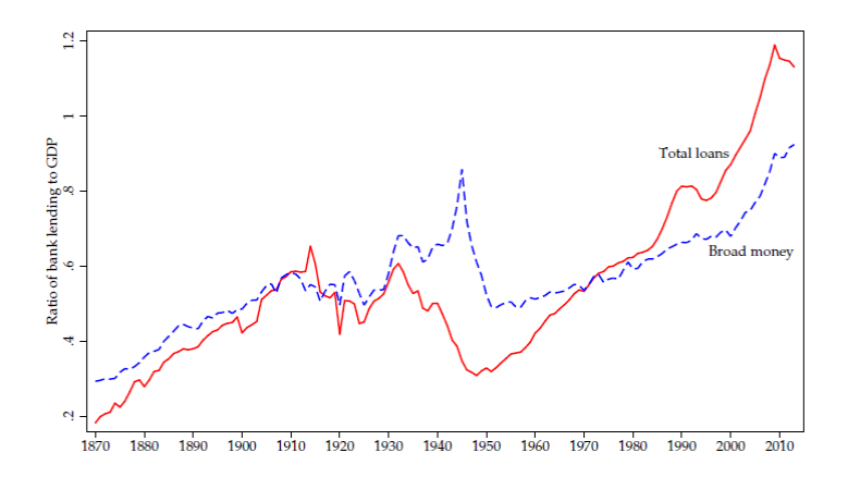
Average ratio of bank loans to the non-financial private sector to GDP across 17 advanced countries (in red) and ratio of M2 to GDP (blue). Source: Jorda, Schularick and Taylor (2016).

This growth in credit was concentrated in mortgage loans as opposed to unsecured lending to businesses.

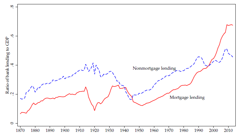
Average ratio of mortgage lending to GDP (red) and for other lending (blue). Source: Jorda, Schularick and Taylor (2016).

This “hockey stick” in mortgage lending was accompanied by a similar pattern in real house prices. These too had been largely stable for nearly a century. Since 1950, house prices have grown faster than inflation around the world.

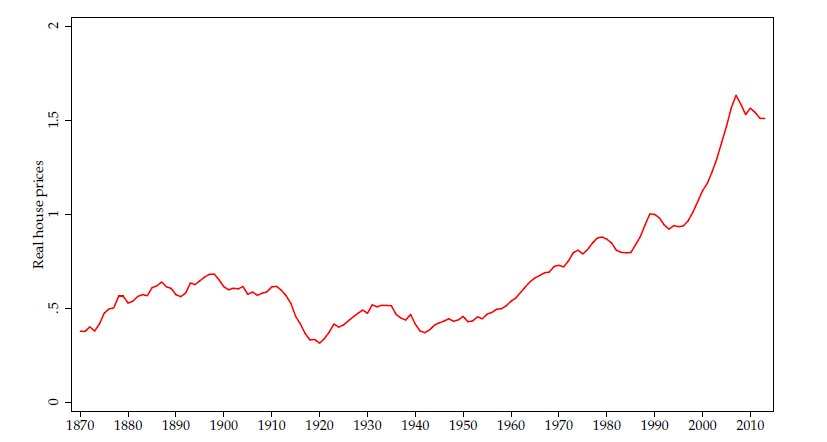
Average house price deflated by CPI across 14 advanced countries. Source: Jorda, Schularick and Taylor (2016).

The authors find that as economies have become more leveraged, the standard deviation of output growth has become smaller, consistent with a phenomenon that has been described as the Great Moderation in the United States since 1985. Interestingly, however, the standard deviation of stock prices has increased. They also find that the skewness of GDP has become more negative– big movements up have become more subdued relative to downturns.

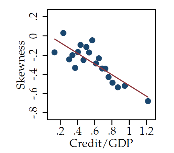
Vertical axis: skewness of GDP within country i over a 10-year period. Horizontal axis: credit/GDP for that country over that period. Data summarized in terms of 20 bins. Source: Jorda, Schularick and Taylor (2016).

The authors conclude:

At a basic level, our core result– that higher leverage goes hand in hand with less volatility, but more severe tail events– is compatible with the idea that expanding private credit may be safe for small shocks, but dangerous for big shocks. Put differently, leverage may expose the system to bigger, rare-event crashes, but it may help smooth more routine, small disturbances.

Guest Contribution: “The Threat to US Global Leadership”

Today we are pleased to present a guest contribution written by Jeffrey Frankel, Harpel Professor of Capital Formation and Growth at Harvard University, and former Member of the Council of Economic Advisers, 1997-99. This is an extended version of a column that appeared in Project Syndicate.

President Barack Obama has had a series of foreign policy triumphs over the last 12 months. One of the lesser-known was the passage of legislation for reform of the IMF on December 18, 2015, after five years of obstruction by the US Congress. As the IMF convenes in Washington DC for its annual spring meetings April 15-17, we should pause to savor the importance of this achievement. One could almost say that if Americans had let yet another year go by without ratifying the IMF quota reform, they might as well have handed over the keys of global economic leadership to someone else. That would be China.

The IMF reform was an important step in updating the allocations of quotas among member countries. (Quota allocations in the IMF determine both monetary contributions of the member states and their voting power. They are supposed to be determined by economic weight.) The agreement among the IMF members was to allocate greater shares to China, India, Brazil and other emerging market countries, coming primarily at the expense of European and Persian Gulf countries. The change in IMF quotas is a partial and overdue adjustment in response to the rise of the newcomers. President Obama managed to get the leaders of the other G20 countries to agree to this reform at a 2010 summit in Seoul.

Approving the agreement should have been a “no-brainer” from the viewpoint of the United States: it was neither to pay a higher budget share nor to lose the voting weight that has always given it a unique veto power in the institution. The reform was an opportunity to exercise US global leadership. But one might have thought it was a threat to US leadership if one judged from congressional opponents who blocked passage of the legislation until last December.

If the game is a competition between China and the US for international power and influence, then some damage has already been done. China feels that its economic success merits a greater role on the world stage. If the status quo powers “move the goal posts” by denying China the place at the table of global governance that it has earned, it will look to establish its own institutions. Meanwhile, Asia has been wondering if the US is committed to the region (as its “pivot” claimed). Indeed, the rest of the world has often in recent years wondered if internal politics prevents the US from functioning at all. Asians tend to prefer to have the US engaged. China’s territorial assertions in the South China Sea confirm its neighbors worst fears. But they will look elsewhere if need be.

Thus Asian countries (and others) were happy to join a new China-led institution, the Asian Infrastructure Investment Bank. The AIIB, widely viewed as a serious diplomatic setback for the US, went into operation December 25.

The good news is that the AIIB is off to a good start, with no sign so far of the feared lowering of standards relative to other multilateral development banks (such as the World Bank). But it is even better news that the US can now get back into the game, after a string of international successes.

It has been a busy 12 months for President Obama in the international arena. Consider global achievements in four areas (in addition to the IMF reform):



On April 2, 2015, the United States (and five other major powers) reached a long-shot breakthrough with Iran over its nuclear program, which was then consummated in a July 14 agreement diverting Tehran from what had seemed an inexorable march to nuclear weapons. On January 16, 2016, the International Atomic Energy Agency verified that Iran had in fact completed the necessary steps under the agreement to ensure that its program remains exclusively peaceful.

On June 24, 2015, Congress was persuaded to give the White House Trade Promotion Authority. It allowed the administration to complete the Trans-Pacific Partnership (TPP) in October.

On July 20, 2015, the US and Cuba re-opened embassies in each other’s countries. Last month, on March 20, Obama because the first president to visit Cuba in 90 years. The historic event marked the end of 55 years of an attempted isolation policy that had only succeeded in giving the Castro brothers an excuse for economic failure and in handicapping American relations throughout Latin America.

On December 12, against all expectations, representatives of 195 parties to the UN Framework Convention on Climate Change successfully reached an agreement on global action in Paris, spurred in no small part by an earlier breakthrough between President Obama and Chinese President Xi Jin Ping. This month, on April 22, the two leaders are scheduled to sign the Paris Agreement on behalf of their respective countries, the world’s two largest emitters of greenhouse gases. The signing will encourage others to ratify.



These accomplishments are not the kind that come automatically with possession of the Oval Office. A year ago, not one of them was expected. Not only did the international political obstacles appear nearly insurmountable; the domestic obstacles looked even worse. The overwhelming conventional wisdom was that Obama would not be able to accomplish much in his remaining time in office. After all, the Republicans had succeeded in blocking almost all Obama’s proposals since they took the House of Representatives in November 2010. Why should he have any better luck after they took the Senate (in November 2014) and especially now that he was a “lame duck” as well?

The Trade Promotion Authority legislation was declared virtually dead last May. The IMF quota reform legislation was considered so moribund, the press did even consider it worth reporting on.

A lot of the opposition came from Republicans who from the start have been eager to line up on the opposite side of whatever position President Obama takes. But opposition to such internationalism comes from the far left of the political spectrum as well as the far right, and not just in the area of trade. To take the salient example of Bernie Sanders, historically he has joined with congressional Republicans in trying to block efforts to rescue emerging market countries in Latin America and Asia at times of financial crisis. (These rescues are invariably called “bailouts,” even while they cost the US nothing – the Treasury made a profit on the 1995 loan to Mexico that Sanders fought – and even while they sustain economic growth.) To take another example, New York Senator Chuck Schumer joined the Republicans in trying to block the Iran nuclear agreement, an effort that failed on September 8.

The IMF deal is done. Managing Director Christine Lagarde is doing a good job (especially compared to her three predecessors, none of whom was even able to serve out his term). She is right, for example, to tell the Germans that a solution to the Greek problem requires further debt-reduction as one of its components.

But each of the other four initiatives could still be de-railed by US politics, especially if the far left and the far right join together. Congress has yet to repeal the Cuba embargo. It could reject the TPP, in effect telling Asia it is on its own. On June 2, a federal Appeals Court will hear a challenge to the Clean Power Plan whereby the Obama Administration hopes to begin implementing its commitment under the Paris Agreement. Donald Trump and Ted Cruz both say that if elected president they would tear up the Iran nuclear deal. (What would happen then? Probably the same thing that happened when George W. Bush took office in 2001 and tore up Bill Clinton’s “framework agreement” with the North Koreans: they predictably and promptly got a bomb.)

The struggle over whether the US will lead the world continues. It is not a struggle between the US and rivals, but a struggle within American politics.

This post written by Jeffrey Frankel.