
Allen B. Downey's Blog: Probably Overthinking It, page 20
March 18, 2016
The retreat from religion is accelerating
Since I started following this trend it 2008, I have called it "one of the most under-reported stories of the decade". I'm not sure if that's true any more; there have been more stories recently about secularization in the U.S., and the general disengagement of Millennials from organized religion.
But one part of the story continues to surprise me: the speed of the transformation is remarkable, averaging almost 1 percentage point per year for the last 20 years, and there is increasing evidence that it is accelerating.
30% have no religion
Among first-year college students in Fall 2015, the fraction reporting no religious affiliation reached an all-time high of 29.6%, up more than 2 percentage points from 27.5% last year.
And the fraction reporting that they never attended a religious service also reached an all-time high at 30.5%, up from 29.3% last year.
These reports are based on survey results from the Cooperative Institutional Research Program (CIRP) of the Higher Education Research Insitute (HERI). In 2015, more than 141,000 full-time, first-time college students at 199 colleges and universities completed the CIRP Freshman Survey, which includes questions about students’ backgrounds, activities, and attitudes.
In one question, students select their “current religious preference,” from a choice of seventeen common religions, “Other religion,” "Atheist", "Agnostic", or “None.” The options "Atheist" and "Agnostic" are new this year. For consistency with previous years, I compare the "Nones" from previous years with the sum of "None", "Atheist" and "Agnostic" this year.
Another question asks students how often they “attended a religious service” in the last year. The choices are “Frequently,” “Occasionally,” and “Not at all.” Students are instructed to select “Occasionally” if they attended one or more times.
The following figure shows the fraction of Nones over more than 40 years of the survey.

The blue line shows actual data through 2014; the red line shows a quadratic fit to the data. The dark gray region shows a 90% confidence interval, which represents uncertainty about the parameters of the model. The light gray region shows a 90% predictive interval, which represents uncertainty about the predicted value.
The blue square shows the actual data point for 2015. For the first time since I starting running this analysis, the new data point falls outside the predicted interval.
30% have not attended a religious service
Here is the corresponding plot for attendance at religious services.
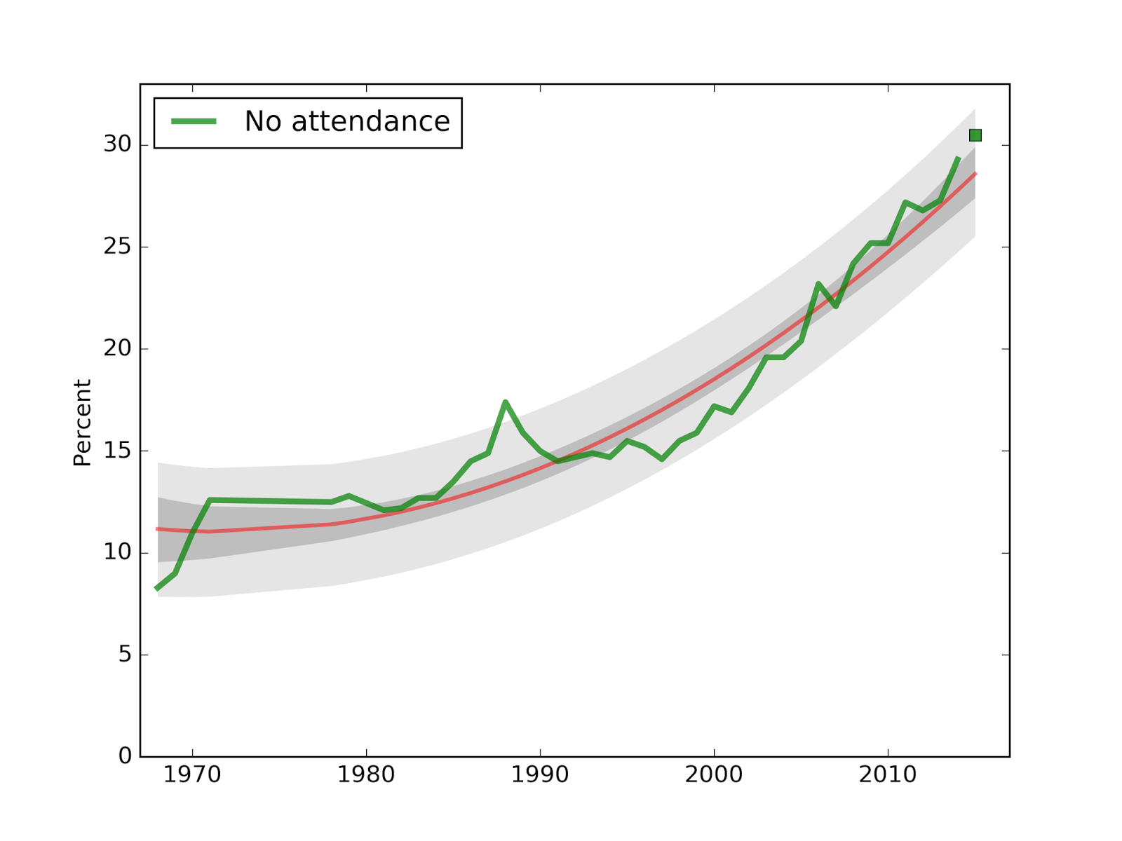
The new data point for 2015, at 30.5%, falls in the predicted range, although somewhat ahead of the long term trend.
The trend is accelerating
The quadratic model suggests that the trend is accelerating, but for a clearer test, I plotted annual changes from 1985 to the present:
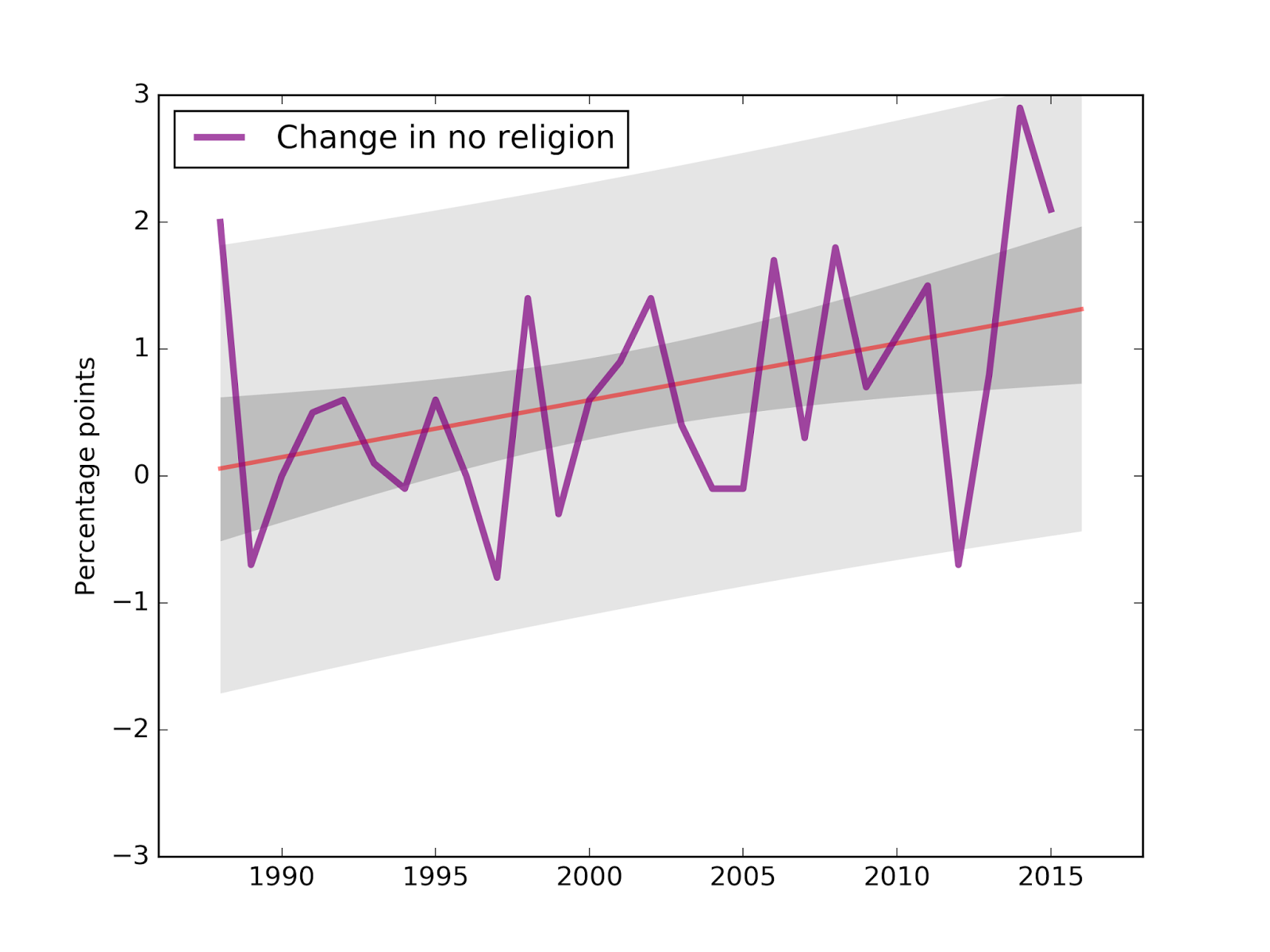 Visually, it looks like the annual changes are getting bigger, and the slope of the fitted line is about 0.4 percentage points per decade. The p-value of that slope is 3.6%, which is considered statistically significant, but barely. You can interpret that as you like.
The gender gap persists
As always, more males than females report no religious preference.
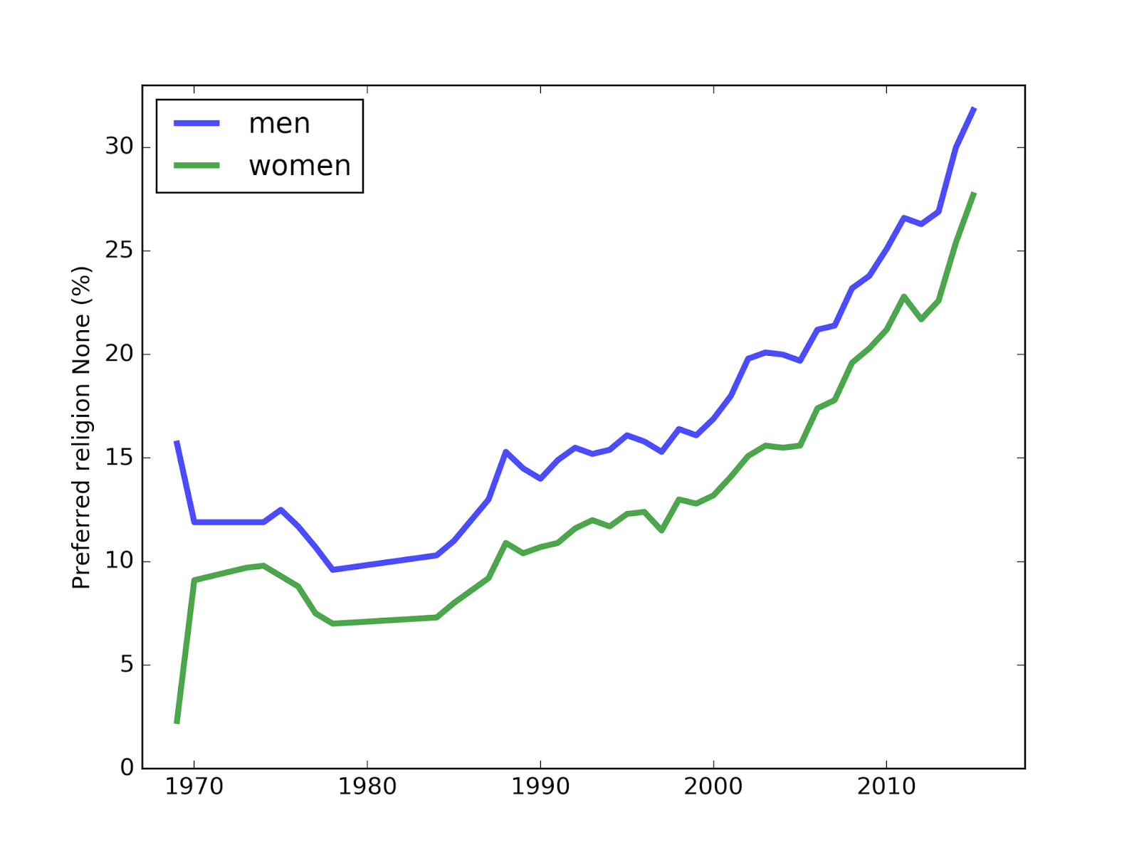 The gender gap closed slightly this year, but the long term trend suggests it is still growing.
Predictions for 2016
Using the new 2015 data, we can run the same analysis to generate predictions for 2016. Here is the revised plot for "Nones":
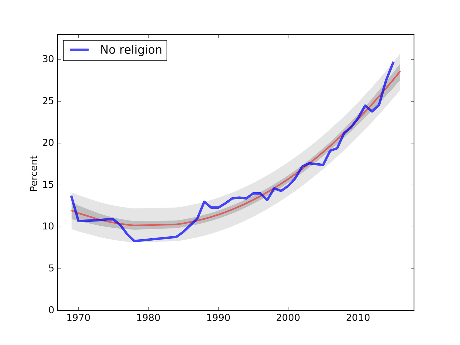
This year's measurement is ahead of the long-term trend, so next year's is predicted to regress to 28.6% (down 1.0%).
And here is the prediction for "No attendance":
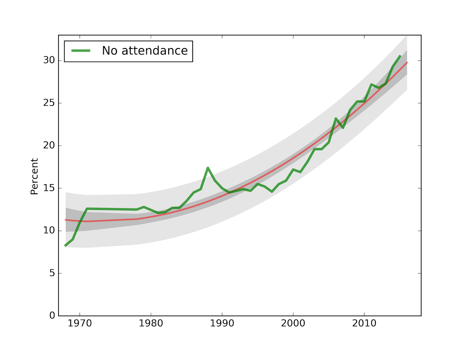
Again, because this year's value is ahead of the long term trend, the center of the predictive distribution is lower, at 29.8% (down 0.7%).
I'll be back next year to check on these predictions.
Comments
1) The addition of the two new categories, "Atheist" and "Agnostic" is new this year. Of the 29.6% I am treating as "no religion", 8.3% reported as agnostic, 5.9% as atheist, and 15.4% as none. It's hard to say what effect the change in the question had on the results.
2) The number of schools and the number of students participating in the Freshman Survey has been falling for several years. I wonder if the mix of schools represented in the survey is changing over time, and what effect this might have on the trends I am watching. The percentage of "Nones" is different across different kinds of institutions (colleges, universities, public, private, etc.) If participation rates are changing among these groups, that would affect the results.
3) Obviously college students are not representative of the general population. Data from other sources indicate that the same trends are happening in the general population, but I haven't been able to make a quantitative comparison between college students and others. Data from other sources also indicate that college graduates are slightly more likely to attend religious services, and to report a religious preference, than the general population.
Data Source
Eagan, K., Stolzenberg, E. B., Ramirez, J. J., Aragon, M. C., Suchard, M. R., & Hurtado, S. (2014). The American freshman: National norms fall 2014. Los Angeles: Higher Education Research Institute, UCLA.
This and all previous reports are available from the HERI publications page.


March 4, 2016
A quick Bayes problem in IPython
The following problem was submitted to my blog, Probably Overthinking It, by a user named Amit, who wrote:
The following data is about a poll that occurred in 3 states. In state1, 50% of voters support Party1, in state2, 60% of the voters support Party1, and in state3, 35% of the voters support Party1. Of the total population of the three states, 40% live in state1, 25% live in state2, and 35% live in state3. Given that a voter supports Party1, what is the probability that he lives in state2?
My solution follows. First I'll create a suite to represent our prior knowledge. If we know nothing about a voter, we would use the relative populations of the states to guess where they are from.
In [2]: prior = thinkbayes2.Suite({'State 1': 0.4, 'State 2': 0.25, 'State 3': 0.35})prior.Print()
State 1 0.4
State 2 0.25
State 3 0.35
Now if we know a voter supports Party 1, we can use that as data to update our belief. The following dictionary contains the likelihood of the data (supporting Party 1) under each hypothesis (which state the voter is from).
In [3]: likelihood = {'State 1': 0.5, 'State 2': 0.60, 'State 3': 0.35}To make the posterior distribution, I'll start with a copy of the prior.
The update consists of looping through the hypotheses and multiplying the prior probability of each hypothesis, hypo, by the likelihood of the data if hypo is true.
The result is a map from hypotheses to posterior likelihoods, but they are not probabilities yet because they are not normalized.
In [4]: posterior = prior.Copy()for hypo in posterior:
posterior[hypo] *= likelihood[hypo]
posterior.Print()
State 1 0.2
State 2 0.15
State 3 0.1225
Normalizing the posterior distribution returns the total likelihood of the data, which is the normalizing constant.
In [5]: posterior.Normalize()Out[5]: 0.4725
Now the posterior is a proper distribution:
In [6]: posterior.Print()State 1 0.42328042328
State 2 0.31746031746
State 3 0.259259259259
And the probability that the voter is from State 2 is about 32%.
In [ ]:
December 8, 2015
Many rules of statistics are wrong
The rules I hold in particular contempt are:
The interpretation of p-values: Suppose you are testing a hypothesis, H, so you've defined a null hypothesis, H0, and computed a p-value, which is the likelihood of an observed effect under H0.
According to the conventional wisdom of statistics, if the p-value is small, you are allowed to reject the null hypothesis and declare that the observed effect is "statistically significant". But you are not allowed to say anything about H, not even that it is more likely in light of the data.
I disagree. If we were really not allowed to say anything about H, significance testing would be completely useless, but in fact it is only mostly useless. As I explained in this previous article, a small p-value indicates that the observed data are unlikely under the null hypothesis. Assuming that they are more likely under H (which is almost always the case), you can conclude that the data are evidence in favor of H and against H0. Or, equivalently, that the probability of H, after seeing the data, is higher than it was before. And it is reasonable to conclude that the apparent effect is probably not due to random sampling, but might have explanations other than H.
Correlation does not imply causation: If this slogan is meant as a reminder that correlation does not always imply causation, that's fine. But based on responses to some of my previous work, many people take it to mean that correlation provides no evidence in favor of causation, ever.
I disagree. As I explained in this previous article, correlation between A and B is evidence of some causal relationship between A and B, because you are more likely to observe correlation if there is a causal relationship than if there isn't. The problem with using correlation for to infer causation is that it does not distinguish among three possible relationships: A might cause B, B might cause A, or any number of other factors, C, might cause both A and B.
So if you want to show that A causes B, you have to supplement correlation with other arguments that distinguish among possible relationships. Nevertheless, correlation is evidence of causation.
Regression provides no evidence of causation: This rule is similar to the previous one, but generalized to include regression analysis. I posed this question the reddit stats forum: the consensus view among the people who responded is that regression doesn't say anything about causation, ever. (More about that in this previous article.)
I disagree. It think regression provides evidence in favor of causation for the same reason correlation does, but in addition, it can distinguish among different explanations for correlation. Specifically, if you think that a third factor, C, might cause both A and B, you can try adding a variable that measures C as an independent variable. If the apparent relationship between A and B is substantially weaker after the addition of C, or if it changes sign, that's evidence that C is a confounding variable.
Conversely, if you add control variables that measure all the plausible confounders you can think of, and the apparent relationship between A and B survives each challenge substantially unscathed, that outcome should increase your confidence that either A causes B or B causes A, and decrease your confidence that confounding factors explain the relationship.
By providing evidence against confounding factors, regression provides evidence in favor of causation, but it is not clear whether it can distinguish between "A causes B" and "B causes A". The received wisdom of statistics says no, of course, but at this point I hope you understand why I am not inclined to accept it.
In this previous article, I explore the possibility that running regressions in both directions might help. At this point, I think there is an argument to be made, but I am not sure. It might turn out to be hogwash. But along the way, I had a chance to explore another bit of conventional wisdom...
Methods for causal inference, like matching estimators, have a special ability to infer causality: In this previous article, I explored a propensity score matching estimator, which is one of the methods some people think have special ability to provide evidence for causation. In response to my previous work, several people suggested that I try these methods instead of regression.
Causal inference, and the counterfactual framework it is based on, is interesting stuff, and I look forward to learning more about it. And matching estimators may well squeeze stronger evidence from the same data, compared to regression. But so far I am not convinced that they have any special power to provide evidence for causation.
Matching estimators and regression are based on many of the same assumptions and vulnerable to some of the same objections. I believe (tentatively for now) that if either of them can provide evidence for causation, both can.
Quoting rules is not an argumentAs these examples show, many of the rules of statistics are oversimplified, misleading, or wrong. That's why, in many of my explorations, I do things experts say you are not supposed to do. Sometimes I'm right and the rule is wrong, and I write about it here. Sometimes I'm wrong and the rule is right; in that case I learn something and I try to explain it here. In the worst case, I waste time rediscovering something everyone already "knew".
If you think I am doing something wrong, I'd be interested to hear why. Since my goal is to test whether the rules are valid, repeating them is not likely to persuade me. But if you explain why you think the rules are right, I am happy to listen.

December 3, 2015
Internet use and religion, part six
I discuss this question in the next section, which is probably too long. If you get bored, you can skip to the following section, which presents a different method for estimating effect size, a "propensity score matching estimator", and compares the results to the regression models.
What does "evidence" mean?In the previous article I presented results from two regression models and made the following argument:
Internet use predicts religiosity fairly strongly: the effect size is stronger than education, income, and use of other media (but not as strong as age).Controlling for the same variables, religiosity predicts Internet use only weakly: the effect is weaker than age, date of interview, income, education, and television (and about the same as radio and newspaper).This asymmetry suggests that Internet use causes a decrease in religiosity, and the reverse effect (religiosity discouraging Internet use) is weaker or zero.It is still possible that a third factor could cause both effects, but the control variables in the model, and asymmetry of the effect, makes it hard to come up with plausible ideas for what the third factor could be.
I am inclined to consider these results as evidence of causation (and not just a statistical association).
When I make arguments like this, I get pushback from statisticians who assert that the kind of observational data I am working with cannot provide any evidence for causation, ever. To understand this position better, I posted this query on reddit.com/r/statistics. As always, I appreciate the thoughtful responses, even if I don't agree. The top-rated comments came from /u/Data_Driven_Dude, who states this position:
Causality is almost wholly a factor of methodology, not statistics. Which variables are manipulated, which are measured, when they're measured/manipulated, in what order, and over what period of time are all methodological considerations. Not to mention control/confounding variables.
So the most elaborate statistics in the world can't offer evidence of causation if, for example, a study used cross-sectional survey design. [...]
Long story short: causality is a helluva lot harder than most people believe it to be, and that difficulty isn't circumvented by mere regression.I believe this is a consensus opinion among many statisticians and social scientists, but to be honest I find it puzzling. As I argued in this previous article, correlation is in fact evidence of causation, because observing a correlation is more likely if there is causation than if there isn't.
The problem with correlation is not that it is powerless to demonstrate causation, but that a simple bivariate correlation between A and B can't distinguish between A causing B, B causing A, or a confounding variable, C, causing both A and B.
But regression models can. In theory, if you control for C, you can measure the causal effect of A on B. In practice, you can never know whether you have identified and effectively controlled for all confounding variables. Nevertheless, by adding control variables to a regression model, you can find evidence for causation. For example:
If A (Internet use, in my example) actually causes B (decreased religiosity), but not the other way around, and we run regressions with B as a dependent variable, and A as an explanatory variable, we expect find that A predicts B, of course. But we also expect the observed effect to persist as we add control variables. The magnitude of the effect might get smaller, but if we can control effectively for all confounding variables, it should converge on the true causal effect size.On the other hand, if we run the regression the other way, using B to predict A, we expect to find that B predicts A, but as we add control variables, the effect should disappear, and if we control for all confounding variables, it should converge to zero.
For example, in this previous article, I found that first babies are lighter than others, by about 3 ounces. However, the mothers of first babies tend to be younger, and babies of younger mothers tend to be lighter. When I control for mother's age, the apparent effect is smaller, less than an ounce, and no longer statistically significant. I conclude that mother's age explains the apparent difference between first babies and others, and that the causal effect of being a first baby is small or zero.
I don't think that conclusion is controversial, but here's the catch: if you accept "the effect disappears when I add control variables" as evidence against causation, then you should also accept "the effect persists despite effective control for confounding variables" as evidence for causation.
Of course the key word is "effective". If you think I have not actually controlled for an important confounding variable, you would be right to be skeptical of causation. If you think the controls are weak, you might accept the results as weak evidence of causation. But if you think the controls are effective, you should accept the results as strong evidence.
So I don't understand the claim that regression models cannot provide any evidence for causation, at all, ever, which I believe is the position my correspondents took, and which seems to be taken as a truism among at least some statisticians and social scientists.
I put this question to /u/Data_Driven_Dude, who wrote the following:
[...]just because you have statistical evidence for a hypothesized relationship doesn't mean you have methodological evidence for it. Methods and stats go hand in hand; the data you gather and analyze via statistics are reflections of the methods used to gather those data.
Say there is compelling evidence that A causes B. So I hypothesize that A causes B. I then conduct multiple, methodologically-rigorous studies over several years (probably over at least a decade). This effectively becomes my research program, hanging my hat on the idea that A causes B. I become an expert in A and B. After all that work, the studies support my hypothesis, and I then suggest that there is overwhelming evidence that A causes B.
Now take your point. There could be nascent (yet compelling) research from other scientists, as well logical "common sense," suggesting that A causes B. So I hypothesize that A causes B. I then administer a cross-sectional survey that includes A, B, and other variables that may play a role in that relationship. The data come back, and huzzah! Significant regression model after controlling for potentially spurious/confounding variables! Conclusion: A causes B.
Nope. In your particular study, ruling out alternative hypotheses by controlling for other variables and finding that B doesn't predict A when those other variables are considered is not evidence of causality. Instead, what you found is support for the possibility that you're on the right track to finding causality. You found that A tentatively predicts B when controlling for XYZ, within L population based on M sample across N time. Just because you started with a causal hypothesis doesn't mean you conducted a study that can yield data to support that hypothesis.
So when I say that non-experimental studies provide no evidence of causality, I mean that not enough methodological rigor has been used to suppose that your results are anything but a starting point. You're tiptoeing around causality, you're picking up traces of it, you see its shadow in the distance. But you're not seeing causality itself, you're seeing its influence on a relationship: a ripple far removed from the source.I won't try to summarize or address this point-by-point, but a few observations:
One point of disagreement seems to be the meaning of "evidence". I admit that I am using it in a Bayesian sense, but honestly, that's because I don't understand any alternatives. In particular, I don't understand the distinction between "statistical evidence" and "methodological evidence".Part of what my correspondent describes is a process of accumulating evidence, starting with initial findings that might not be compelling and ending (a decade later!) when the evidence is overwhelming. I mostly agree with this, but I think the process starts when the first study provides some evidence and continues as each additional study provides more. If the initial study provides no evidence at all, I don't know how this process gets off the ground. But maybe I am still stuck on the meaning of "evidence".A key feature of this position is the need for methodological rigor, which sounds good, but I am not sure what it means. Apparently regression models with observational data lack it. I suspect that randomized controlled trials have it. But I'm not sure what's in the middle. Or, to be more honest, I know what is considered to be in the middle, but I'm not sure I agree.To pursue the third point, I am exploring methods commonly used in the social sciences to test causality.
SKIP TO HERE!Matching estimators of causal effectsI'm reading Morgan and Winship's Counterfactuals and Causal Inference , which is generally good, although it has the academic virtue of presenting simple ideas in complicated ways. So far I have implemented one of the methods in Counterfactuals, a propensity score matching estimator. Matching estimators work like this:
To estimate the effect of a particular treatment, D, on a particular outcome, Y, we divide an observed sample into a treatment group that received D and a control group that didn't.For each member of the treatment group, we identify a member of the control group that is as similar as possible (I'll explain how soon), and compute the difference in Y between the matched pair.Averaging the observed differences over the pairs yields an estimate of the mean causal effect of D on Y.
The hard part of this process is matching. Ideally the matching process should take into account all factors that cause Y. If the pairs are identical in all of these factors, and differ only in D, any average difference in Y must be caused by D.
Of course, in practice we can't identify all factors that cause Y. And even if we could, we might not be able to observe them all. And even if we could, we might not be able to find a perfect match for each member of the treatment group.
We can't solve the first two problems, but "propensity scores" help with the third. The basic idea is
Identify factors that predict D. In my example, D is Internet use.Build a model that uses those factors to predict the probability of D for each member of the sample; this probability is the propensity score. In my example, I use logistic regression with age, income, education, and other factors to compute propensity scores. Match each member of the treatment group with the member in the control group with the closest propensity score. In my example, the members of each pair have the same predicted probability of using the Internet (according to the model in step 2), so the only relevant difference between them is that one did and one didn't. Any difference in the outcome, religiosity, should reflect the causal effect of the treatment, Internet use.I implemented this method (details below) and applied it to the data from the European Social Survey (ESS).
In each country I divide respondents into a treatment group with Internet use above the median and a control group below the median. We lose information by quantizing Internet use in this way, but the distribution tends to be bimodal, with many people at the extremes and few in the middle, so treating Internet use as a binary variable is not completely terrible.
To compute propensity scores, I use logistic regression to predict Internet use based on year of birth (including a quadratic term), year of interview, education and income (as in-country ranks), and use of other media (television, radio, and newspaper).
As expected, the average propensity in the treatment group is higher than in the control group. But some members of the control group are matched more often than others (and some not at all). After matching, the two groups have the same average propensity.
Finally, I compute the pair-wise difference in religiosity and the average across pairs.
For each country, I repeat this process 101 times using weighted resampled data with randomly filled missing values. That way I can compute confidence intervals that reflect variation due to sampling and missing data. The following figure shows the estimated effect size for each country and a 95% confidence interval:
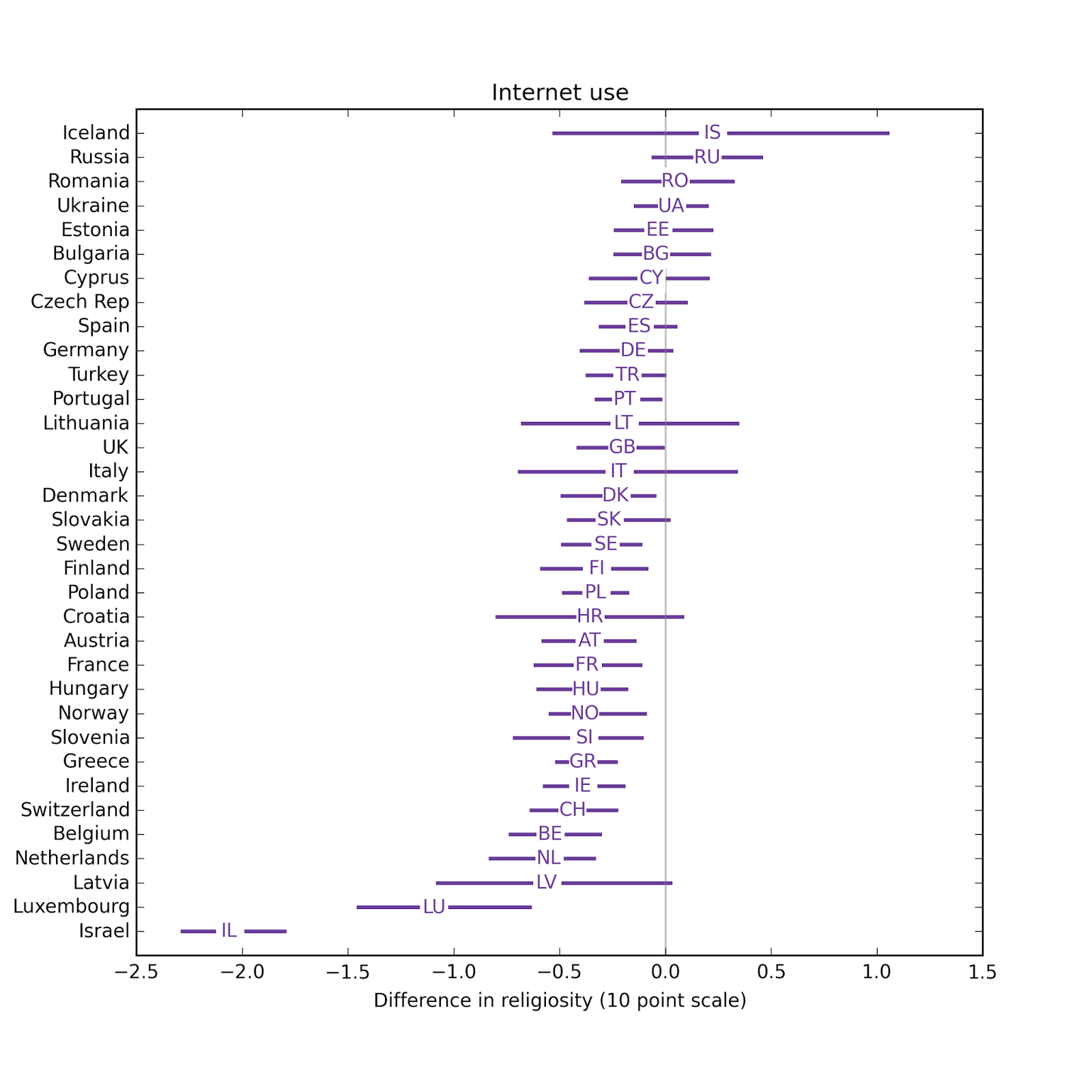 The estimated effect of Internet use on religiosity is negative in 30 out of 34 countries; in 18 of them it is statistically significant. In 4 countries the estimate is positive, but none of them are statistically significant.
The median effect size is 0.28 points on a 10 point scale. The distribution of effect size across countries is similar to the results from the regression model, which has median 0.33:
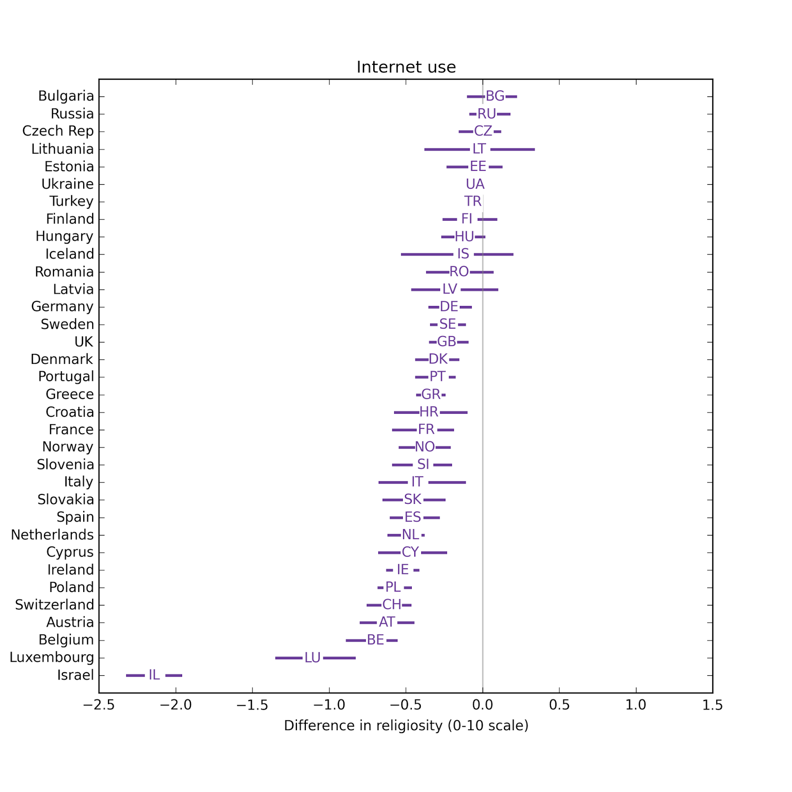
The confidence intervals for the matching estimator are bigger. Some part of this difference is because of the information we lose by quantizing Internet use. Some part is because we lose some samples during the matching process. And some part is due to the non-parametric nature of matching estimators, which make fewer assumptions about the structure of the effect.
How it worksThe details of the method are in this IPython notebook, but I'll present the kernel of the algorithm here. In the following, group is a Pandas DataFrame for one country, with one row for each respondent.
The first step is to quantize Internet use and define a binary variable, treatment:
netuse = group.netuse_f
thresh = netuse.median()
if thresh < 1:
thresh = 1
group.treatment = (netuse >= thresh).astype(int)
The next step is use logistic regression to compute a propensity for each respondent:
formula = ('treatment ~ inwyr07_f + '
'yrbrn60_f + yrbrn60_f2 + '
'edurank_f + hincrank_f +'
'tvtot_f + rdtot_f + nwsptot_f')
model = smf.logit(formula, data=group)
results = model.fit(disp=False)
group.propensity = results.predict(group)
Next we divide into treatment and control groups:
treatment = group[group.treatment == 1]
control = group[group.treatment == 0]
And sort the controls by propensity:
series = control.propensity.sort_values()
Then do the matching by bisection search:
indices = series.searchsorted(treatment.propensity)
indices[indices < 0] = 0
indices[indices >= len(control)] = len(control)-1
And select the matches from the controls:
control_indices = series.index[indices]
matches = control.loc[control_indices]
Extract the distance in propensity between each pair, and the difference in religiosity:
distances = (treatment.propensity.values -
matches.propensity.values)
differences = (treatment.rlgdgr_f.values -
matches.rlgdgr_f.values)
Select only the pairs that are a close match
caliper = differences[abs(distances) < 0.001]
And compute the mean difference:
delta = np.mean(caliper)
That's all there is to it. There are better ways to do the matching, but I started with something simple and computationally efficient (it's n log n, where n is the size of the control or treatment group, whichever is larger).
Back to the philosophyThe agreement of the two methods provides some evidence of causation, because if the effect were spurious, I would expect different methodologies, which are more or less robust against the spurious effect, to yield different results.
But it is not very strong evidence, because the two methods are based on many of the same assumptions. In particular, the matching estimator is only as good as the propensity model, and in this case the propensity model includes the same factors as the regression model. If those factors effectively control for confounding variables, both methods should work. If they don't, neither will.
The propensity model uses logistic regression, so it is based on the usual assumptions about linearity and the distribution of errors. But the matching estimator is non-parametric, so it depends on fewer assumptions about the effect itself. It seems to me that being non-parametric is a potential advantage of matching estimators, but it doesn't help with the fundamental problem, which is that we don't know if we have effectively controlled for all confounding variables.
So I am left wondering why a matching estimator should be considered suitable for causal inference if a regression model is not. In practice one of them might do a better job than the other, but I don't see any difference, in principle, in their ability to provide evidence for causation: either both can, or neither.

November 30, 2015
Internet use and religion, part five
In the previous article, I show results from two regression models that predict religious affiliation and degree of religiosity. I use the models to compare hypothetical respondents who are at their national means for all explanatory factors; then I vary one factor at a time, comparing someone at the 25th percentile with someone at the 75th percentile. I compute the different in the predicted probability of religious affiliation and the predicted level of religiosity:
1) In almost every country, a hypothetical respondent with high Internet use is less likely to report a religious affiliation. The median effect size across countries is 3.5 percentage points.
2) In almost every country, a hypothetical respondent with high Internet use reports a lower degree of religiosity. The median effect size is 0.36 points on a 10-point scale.
These results suggest that Internet use might cause religious disaffiliation and decreased religiosity, but they are ambiguous. It is also possible that the direction of causation is the other way; that is, that religiosity causes a decrease in Internet use. Or there might be other factors that cause both Internet use and religiosity.
I'll address the first possibility first. If religiosity causes lower Internet use, we should be able to measure that effect by flipping the models, taking religious affiliation and religiosity as explanatory variables and trying to predict Internet use.
I did that experiment and found:
1) Religious affiliation (hasrelig) has no predictive value for Internet use in most countries, and only weak predictive value in others.
2) Degree of religiosity (rlgdgr) has some predictive value for Internet use in some countries, but the effect is weaker than other explanatory variables (like age and education), and weaker than the effect of Internet use on religiosity: the median across countries is 0.19 points on a 7-point scale.
Considering the two possibilities, that Internet use causes religious disaffiliation or the other way around, these results support the first possibility, although the second might make a smaller contribution.
Although it is still possible that a third factor causes increased Internet use and decreased religious affiliation, it would have to do so in a strangely asymmetric way to account for these results. And since the model controls for age, income, education, and other media use, this hypothetical third factor would have to be uncorrelated with these controls (or only weakly correlated).
I can't think of any plausible candidates for this third factor. So I tentatively conclude that Internet use causes decreased religiosity. I present more detailed results below.
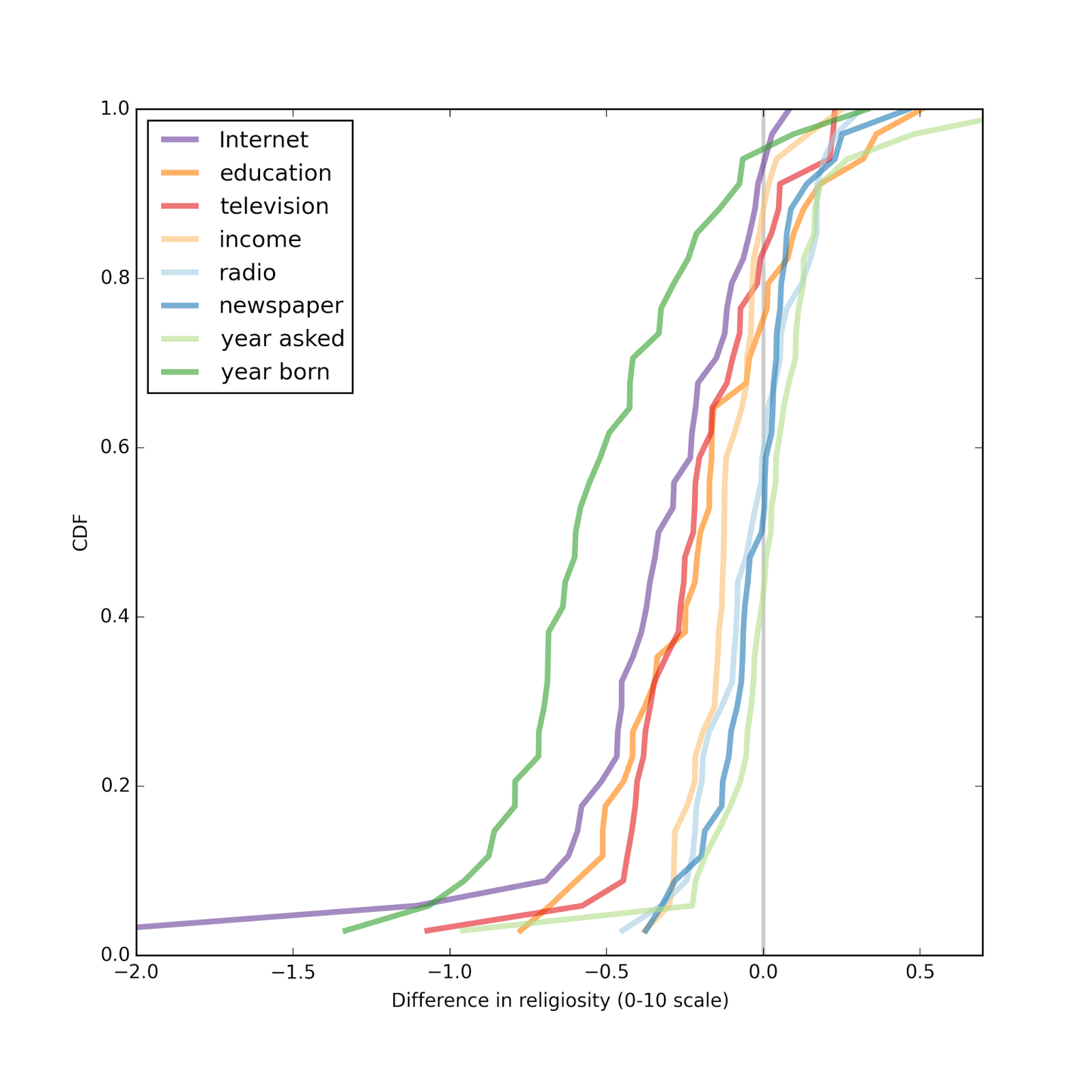
Summary of previous resultsIn the previous article, I computed an effect size for each factor and reported results for two models, one that predicts hasrelig (whether the respondent reports religious affiliations) and one that predicts rlgdgr (degree of religiosity on a 0-10 scale). The following two graphs summarize the results.
Each figure shows the distribution of effect size across the 34 countries in the study. The first figure shows the results for the first model as a difference in percentage points; each line shows the effect size for a different explanatory variable.
The factors with the largest effect sizes are year of birth (dark green line) and Internet use (purple).
For Internet use, a respondent who is average in every way, but falls at the 75th percentile of Internet use, is typically 2-7 percentage points less likely to be affiliated than a similar respondent at the 25th percentile of Internet use. In a few countries, the effect is apparently the other way around, but in those cases the estimated effect size is not statistically significant.
Overall, people who use the Internet more are less likely to be affiliated, and the effect is stronger than the effect of education, income, or the consumption of other media.
Similarly, when we try to predict degree of religiosity, people who use the Internet more (again comparing the 75th and 25th percentiles) report lower religiosity, typically 0.2 to 0.7 points on a 10 point scale. Again, the effect size for Internet use is bigger than for education, income, or other media.
 Of course, what I am calling an "effect size" may not be an effect in the sense of cause and effect. What I have shown so far is that Internet users tend to be less religious, even when we control for other factors. It is possible, and I think plausible, that Internet use actually causes this effect, but there are two other possible explanations for the observed statistical association:
1) Religious affiliation and religiosity might cause decreased Internet use.
2) Some other set of factors might cause both increased Internet use and decreased religiosity.
Addressing the first alternative explanation, if people who are more religious tend to use the Internet less (other things being equal), we would expect that effect to appear in a model that includes religiosity as an explanatory variable and Internet use as a dependent variable.
But it turns out that if we run these models, we find that religiosity has little power to predict levels of Internet use when we control for other factors. I present the results below; the details are in this IPython notebook.
Model 1The first model tries to predict level of Internet use taking religious affiliation (hasrelig) as an explanatory variable, along with the same controls I used before: year of birth (linear and quadratic terms), year of interview, education, income, and consumption of other media.
The following figure shows the effect size of religious affiliation on Internet use.
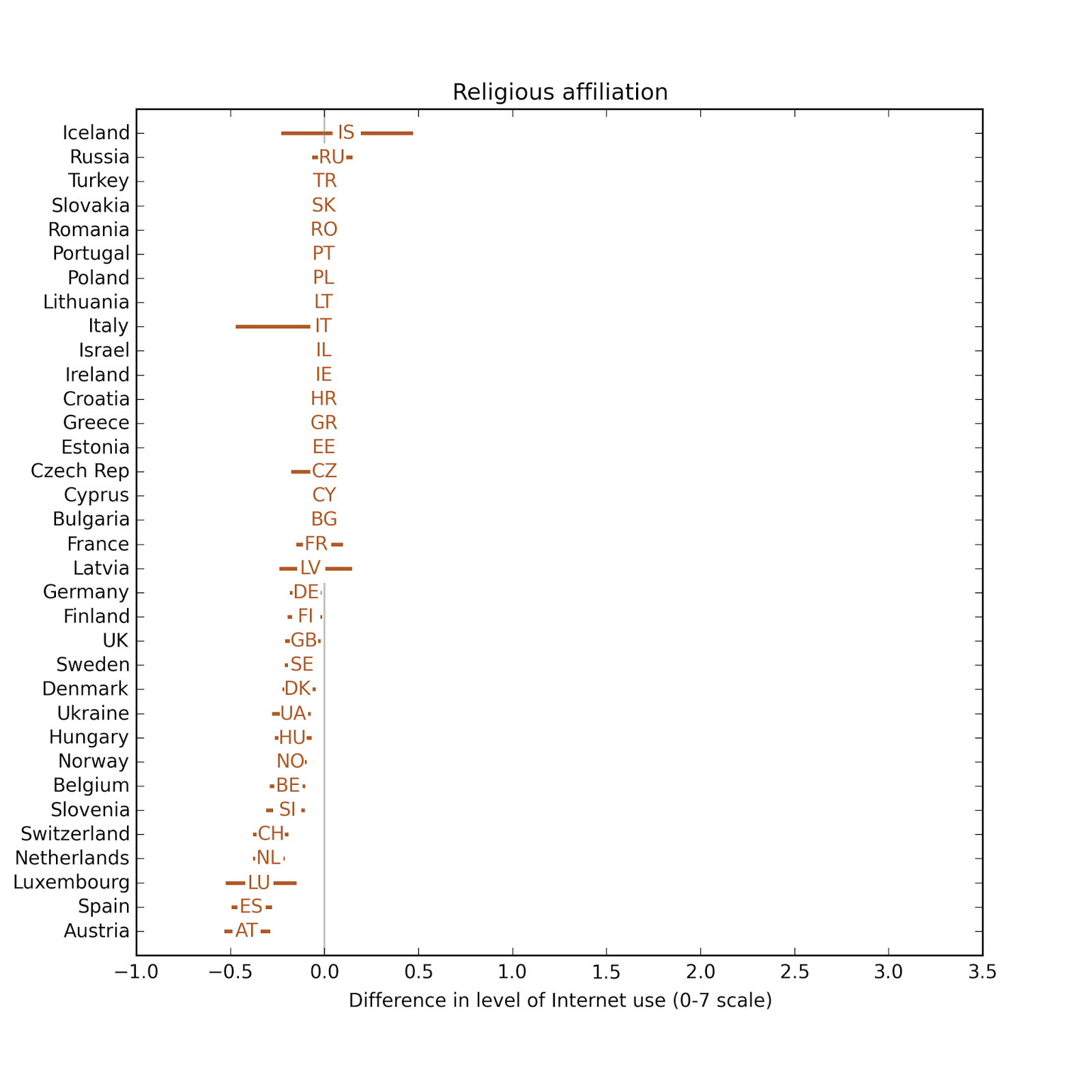 In most countries it is essentially zero, but in a few countries people who report a religious affiliation also report less Internet use, but always less than 0.5 points on a 7 point scale.
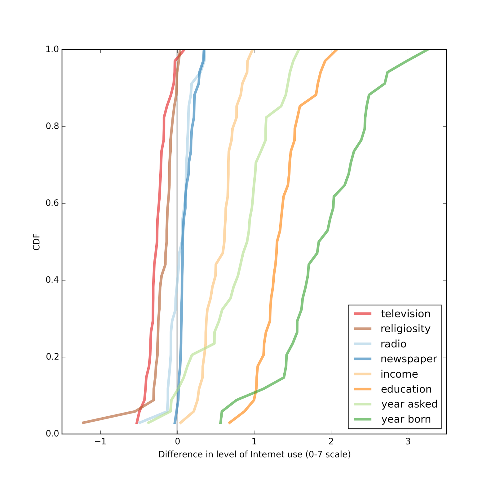
The following figure shows the distribution of effect size for the other variables on the same scale.
 If we are trying to predict Internet use for a given respondent, the most useful explanatory variables, in descending order of effect size, are year of birth, education, year of interview, income, and television viewing. The effect sizes for religious affiliation, radio listening, and newspaper reading are substantially smaller.
The results of the second model are similar.
Model 2The second model tries to predict level of Internet use taking degree of religiosity (rlgdgr) as an explanatory variable, along with the same controls I used before.
The following figure shows the estimated effect size in each country, showing the difference in Internet use of two hypothetical respondents who are at their national mean for all variables except degree of religiosity, where they are at the 25th and 75th percentiles.

In most countries, the respondent reporting a higher level of religiosity also reports a lower level of Internet use, in almost all cases less than 0.5 points on a 7-point scale. Again, this effect is smaller than the apparent effect of the other explanatory variables.
 Again, the variables that best predict Internet use are year of birth, education, year of interview, income, and television viewing. The apparent effect of religiosity is somewhat less than television viewing, and more than radio listening and newspaper reading.
Next stepsAs I present these results, I realize that I can make them easier to interpret by expressing the effect size in standard deviations, rather than raw differences. Internet use is recorded on a 7 point scale, and religiosity on a 10 point scale, so its not obvious how to compare them.
Also, variability of Internet use and religiosity is different across countries, so standardizing will help with comparisons between countries, too.
More results in the next installment.

November 24, 2015
Internet use and religion, part four
As control variables, I include year born, education and income (expressed as relative ranks within each country) and the year the data were gathered (between 2002 and 2010).
Some of the findings so far:
In almost every country, younger people are less religious.In most countries, people with more education are less religious.In about half of the 34 countries, people with lower income are less religious. In the rest, the effect (if any) is too small to be distinguished from noise with this sample size.In most countries, people who watch more television are less religious.In a fewer than half of the countries, people who listen to more radio are less religious.The results for newspapers are similar: only a few countries show a negative effect, and in some countries the effect is positive.In almost every country, people who use the Internet are less religious.There is a weak relationship between the strength of the effect and the average degree of religiosity: the negative effect of Internet use on religion tends to be stronger in more religious countries.In the previous article, I measured effect size using the parameters of the regression models: for logistic regression, the parameter is a log odds ratio, for linear regression it is a linear weight. These parameters are not useful for comparing the effects of different factors, because they are not on the same scale, and they are not the best choice for comparing effect size between countries, because they don't take into account variation in each factor in each country.
For example, in one country the parameter associated with Internet use might be small, but if there is large variation in Internet use within the country, the net effect size might be greater than in another country with a larger parameter, but little variation.
Effect sizeSo my next step is to define effect size in terms that are comparable between factors and between countries. To explain the methodology, I'll use the logistic model, which predicts the probability of religious affiliation. I start by fitting the model to the data, then use the model to predict the probability of affiliation for a hypothetical respondent whose values for all factors are the national mean. Then I vary one factor at a time, generating predictions for hypothetical respondents whose value for one factor is at the 25th percentile (within country) and at the 75th percentile. Finally, I compute the difference in predicted values in percentage points.
As an example, suppose a hypothetically average respondent has a 45% chance of reporting a religious affiliation, as predicted by the model. And suppose the 25th and 75th percentiles of Internet use are 2 and 7, on a 7 point scale. A person who is average in every way, but with Internet use only 2 might have a 47% chance of affiliation. The same person with Internet use 7 might have a 42% chance. In that case I would report that the effect size is a difference of 5 percentage points.
As in the previous article, I run this analysis on about 200 iterations of resampled data, then compute a median and 95% confidence interval for each value.
The IPython notebook for this installment is here.
Quadratic age modelBefore I get to the results, there is one other change from the previous installment: I added a quadratic term for year born. The reason is that in preliminary results, I noticed that Internet had the strongest negative association with religiosity, followed by television, then radio and newspapers. I wondered whether this pattern might be the result of correlation with age; that is, whether younger people are more likely to consume new media and be less religious. I was already controlling for age using yrborn60 (year born minus 1960) but I worried that if the relationship with age is nonlinear, I might not be controlling for it effectively.
So I added a quadratic term to the model. Here are the estimated parameters for the linear term and quadratic term:
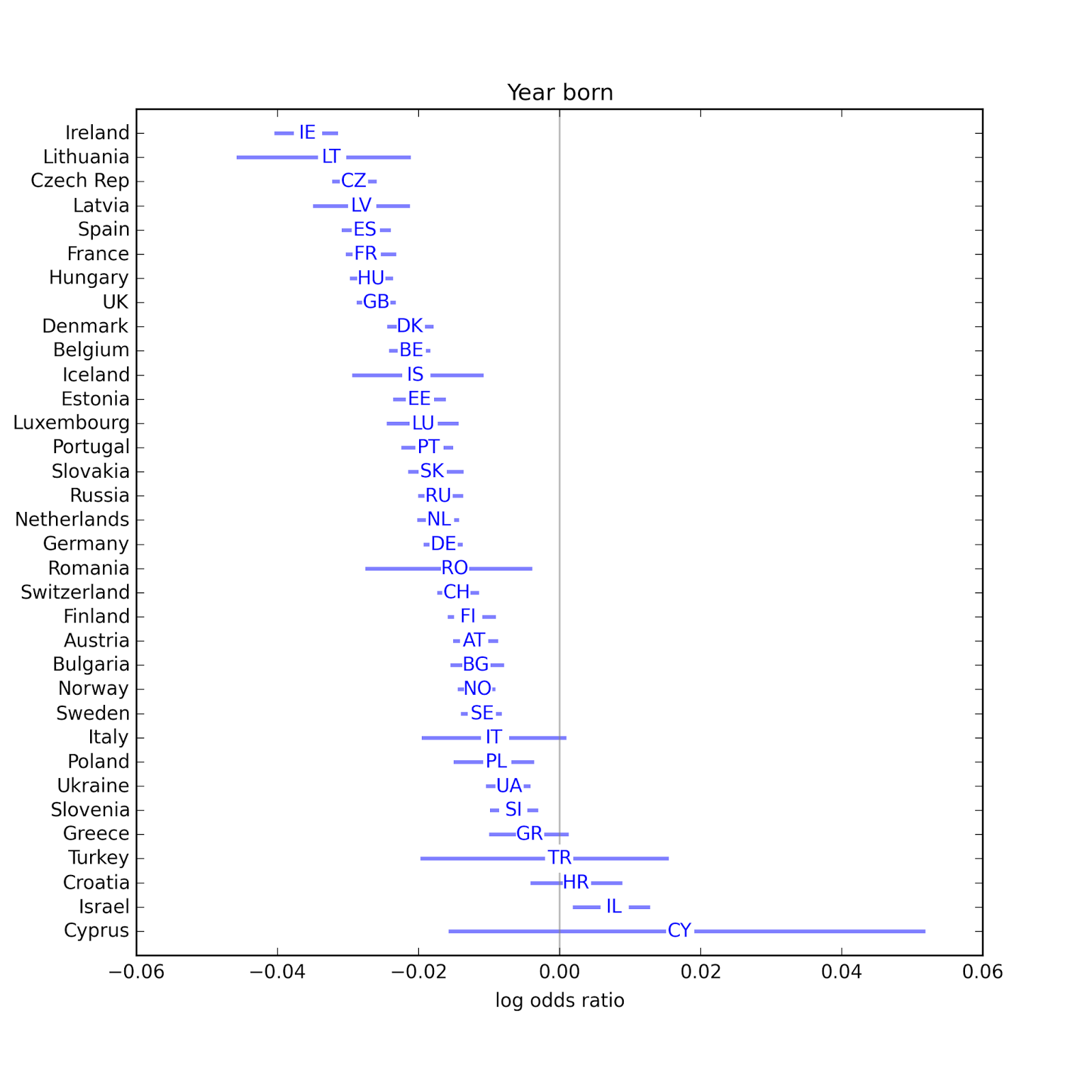
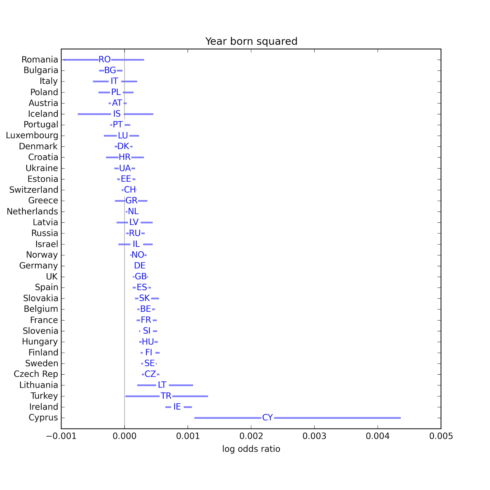 In many countries, both parameters are statistically significant, so I am inclined to keep them in the model. The sign of the quadratic term is usually positive, so the curves are convex up, which suggests that the age effect might be slowing down.
Anyway, including the quadratic term has almost no effect on the other results: the relative strengths of the associations are the same.
Model 1 resultsAgain, the first model uses logistic regression with dependent variable hasrelig, which indicates whether the respondent reports a religious affiliation.
In the following figures, the x-axis is the percentage point difference in hasrelig between people at the 25th and 75th percentile for each explanatory variable.
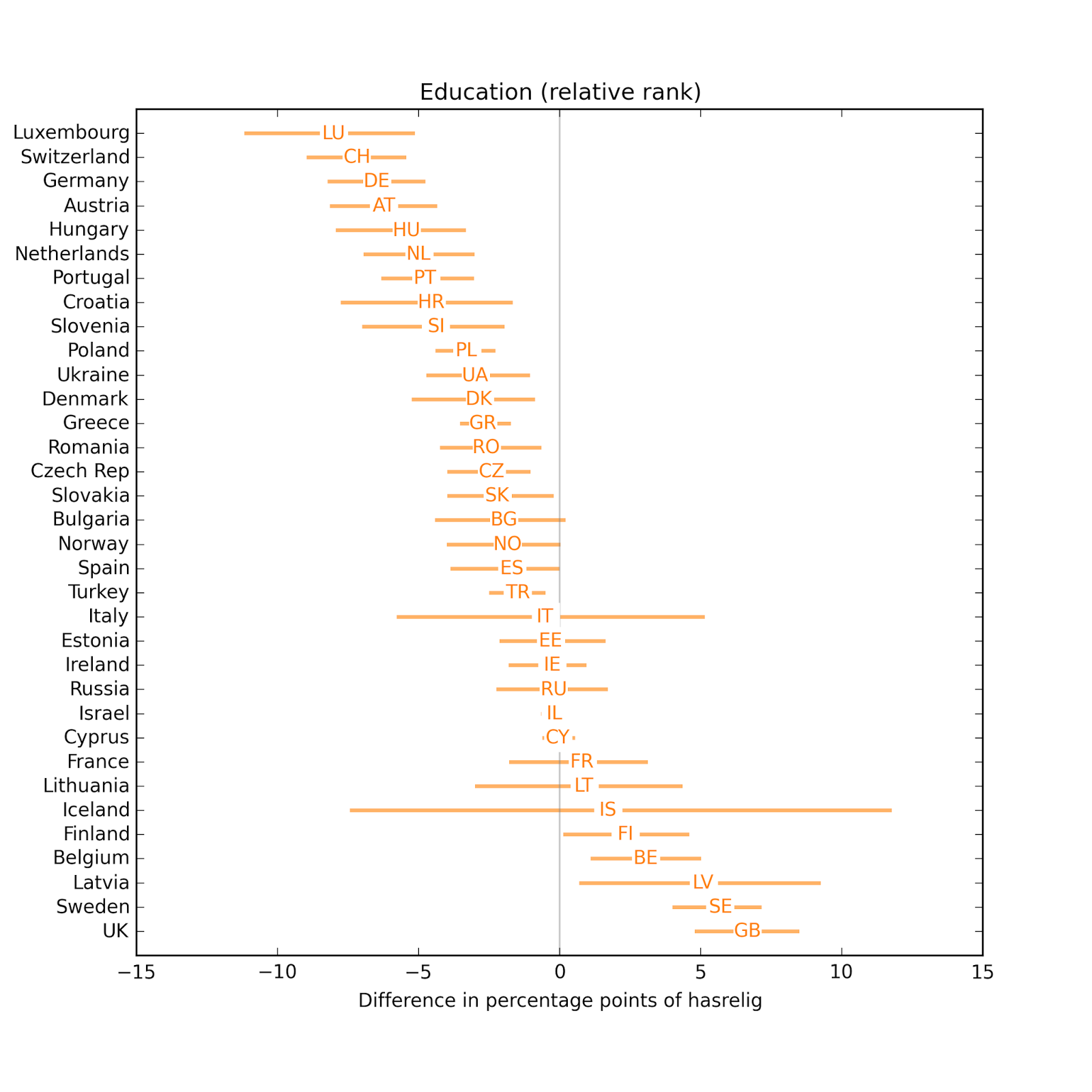 In most countries, people with more education are less religious.
 In most countries, the effect of income is small and not statistically significant.
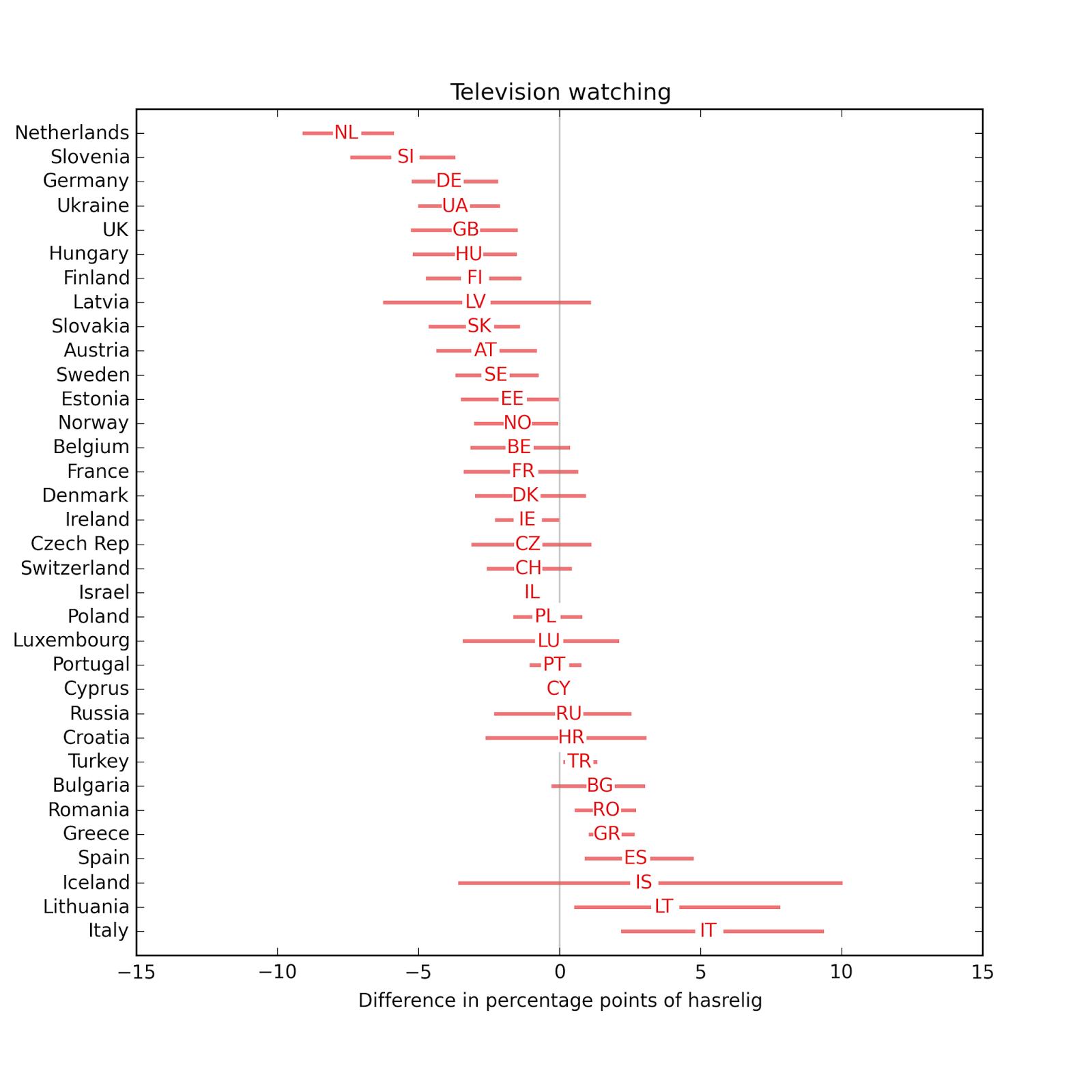 The effect of television is negative in most countries.
 The effect of radio is usually small.
 The effect of newspapers is usually small.
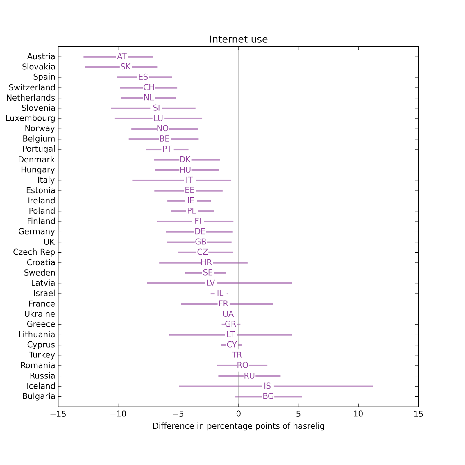 In most countries, Internet use is associated with substantial decreases in religious affiliation.
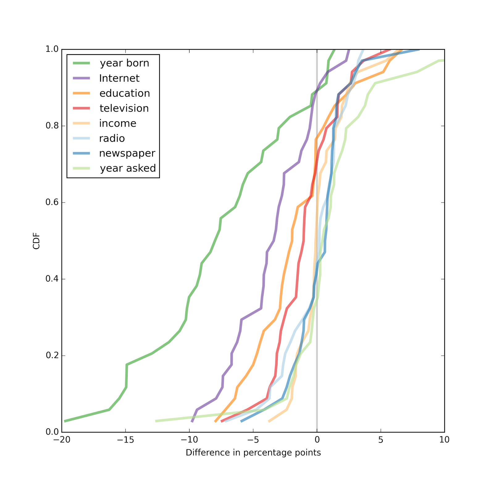
Pulling together the results so far, the following figure shows the distribution (CDF) of effect size across countries:
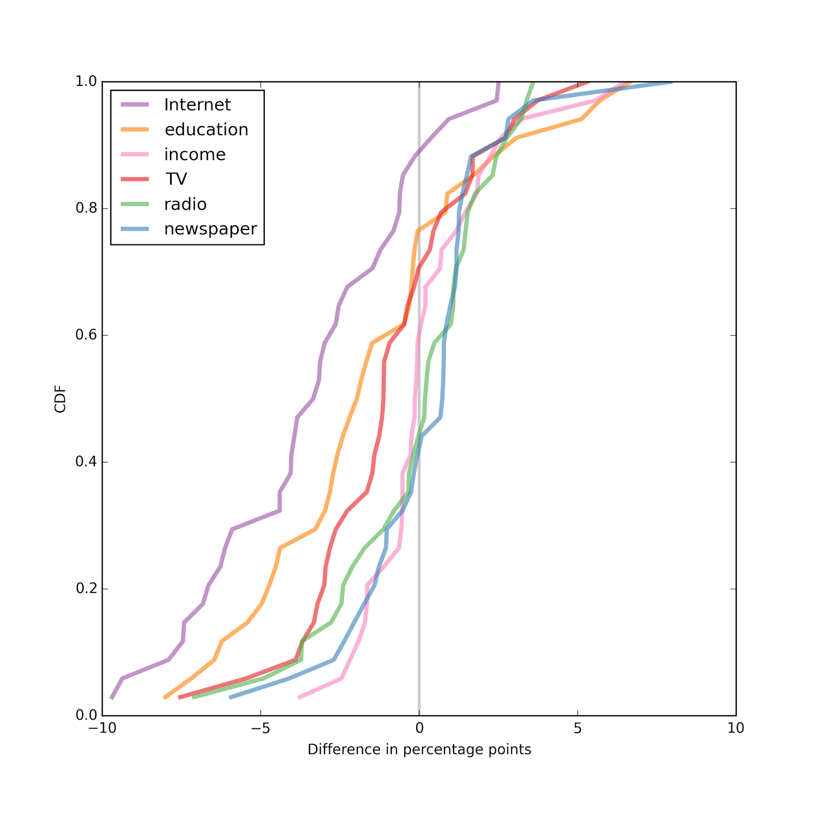 Overall, the effect size for Internet use is the largest, followed by education and television. The effect sizes for income, radio, and newspaper are all small, and centered around zero.
Model 2 resultsThe second model uses linear regression with dependent variable rlgdgr, which indicates degree of religiosity on a 0-10 scale.
In the following figures, the x-axis shows the difference in rlgdgr between people at the 25th and 75th percentile for each explanatory variable.
 In most countries, people with more education are less religious.
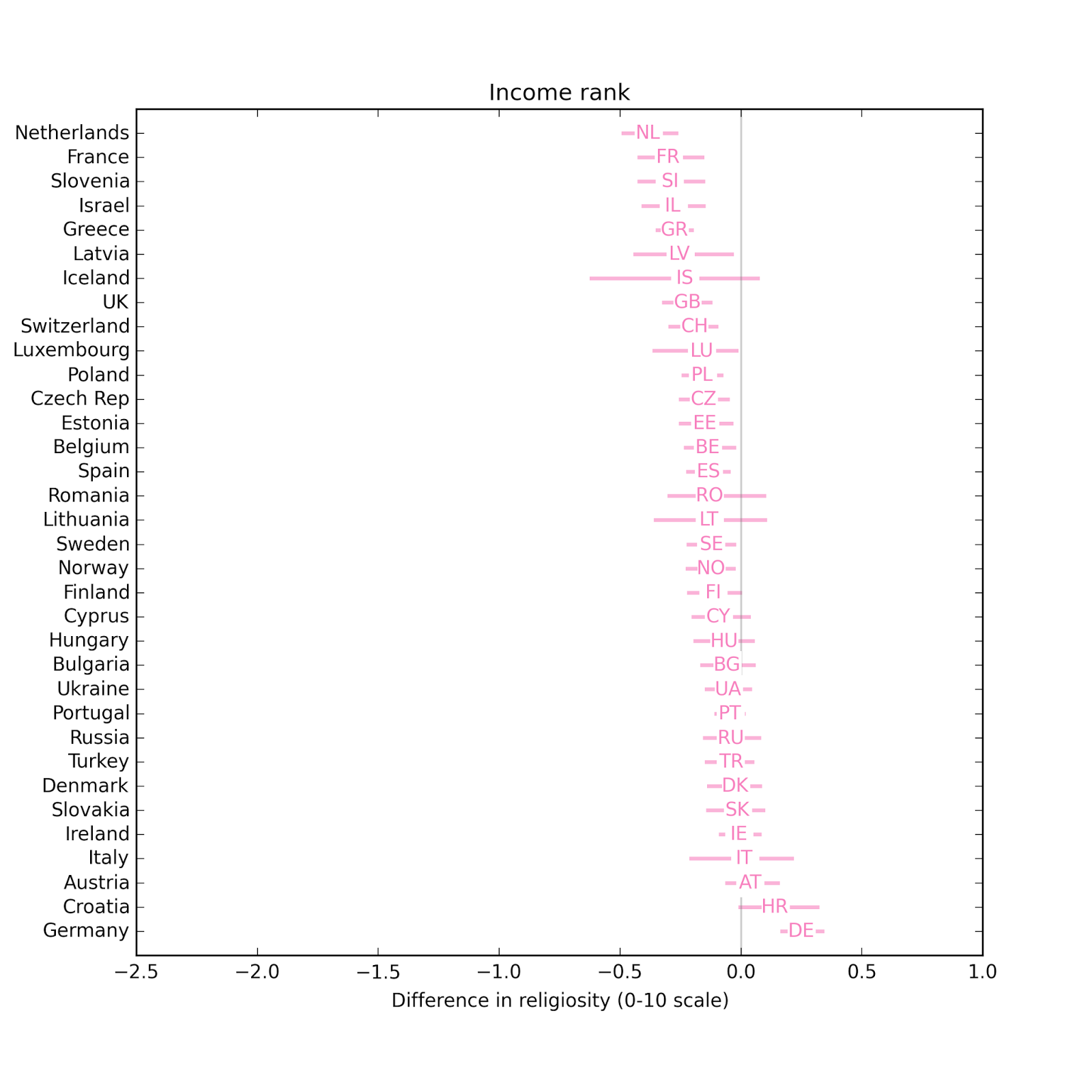 The effect size for income is smaller.
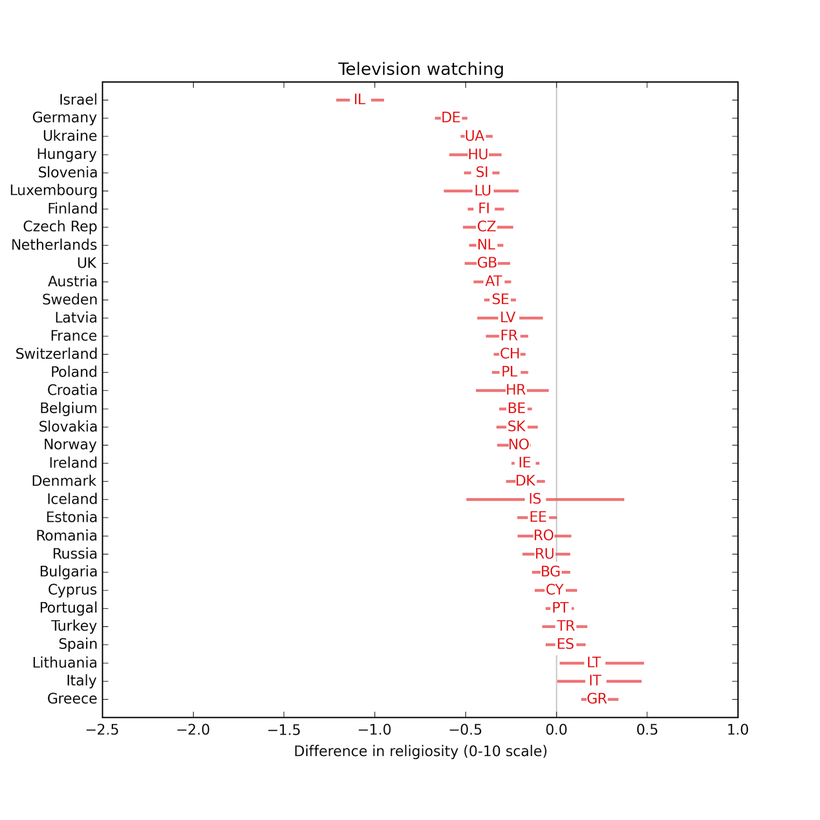 People who watch more television are less religious.
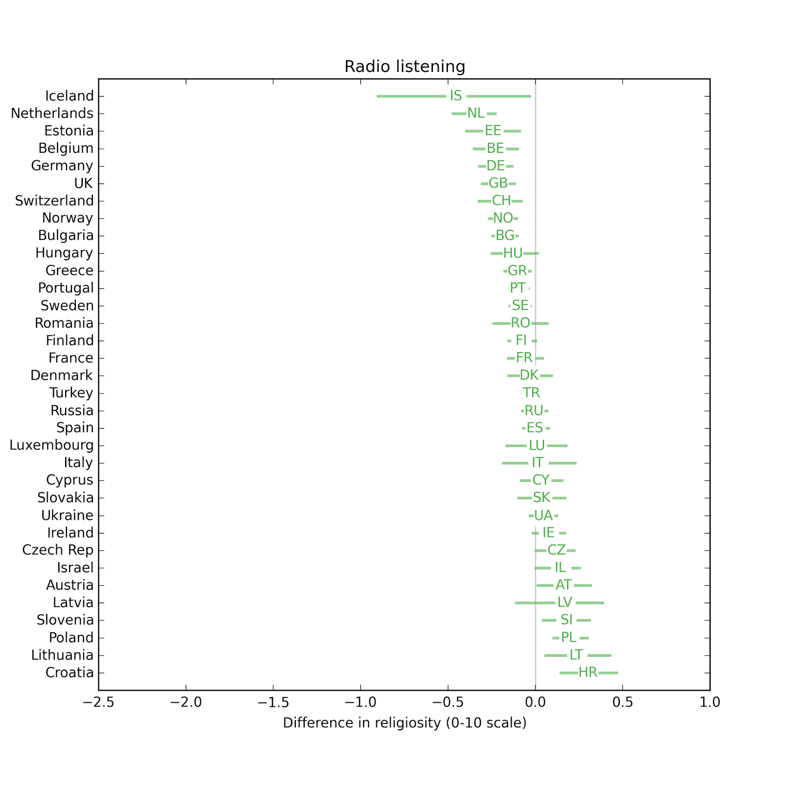 The effect size for radio is small.
 The effect size for newspapers is small.
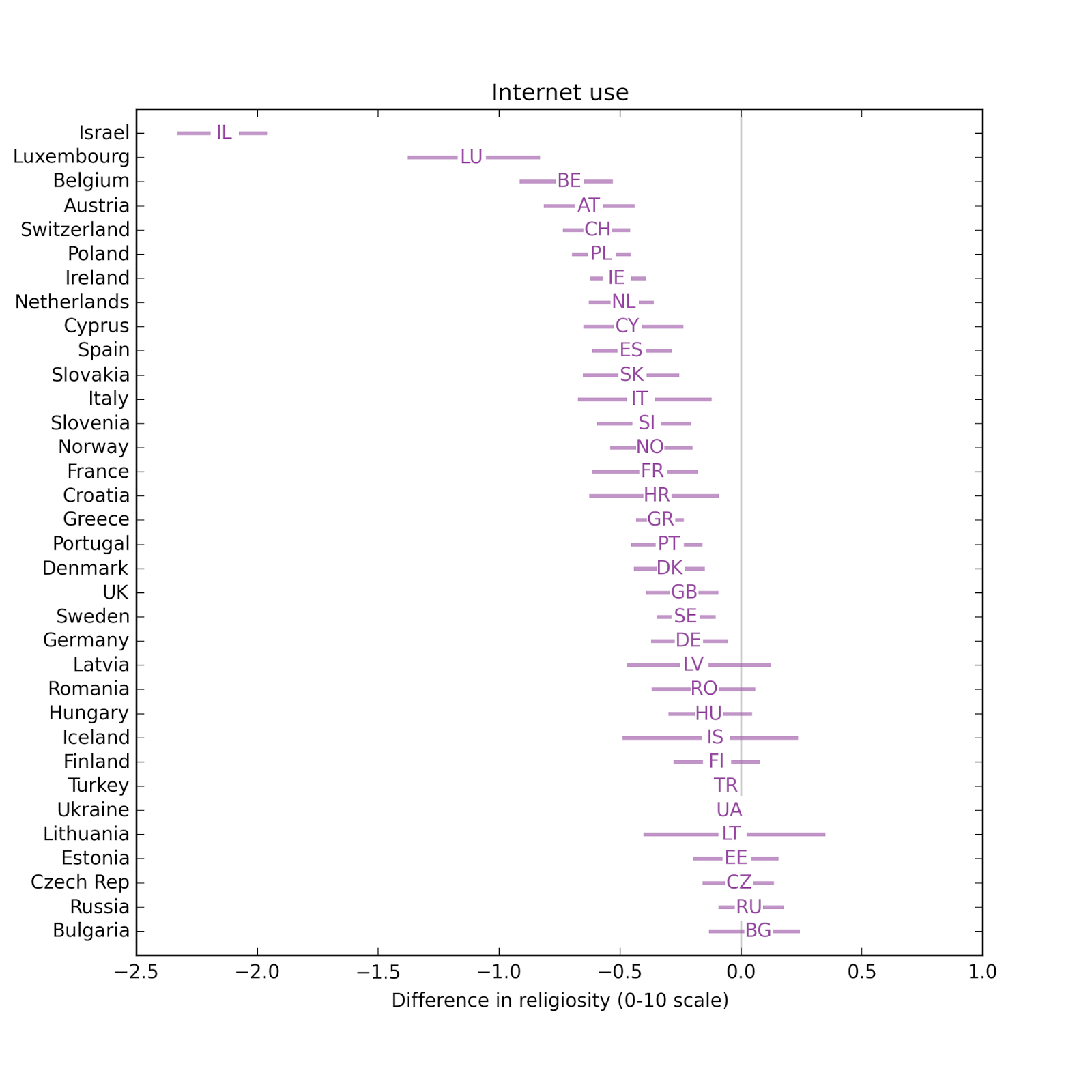 In most countries, people who use the Internet more are less religious.
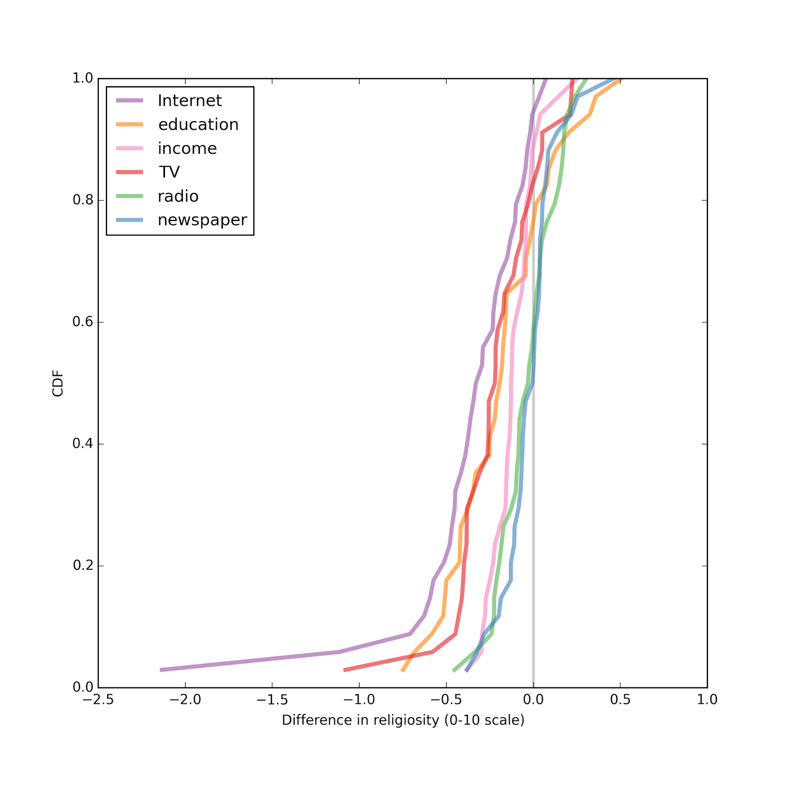 Comparing the effect size for different explanatory variable, again, Internet use has the biggest effect, followed by education and television. Effect sizes for income, radio, and newspaper are smaller and centered around zero.
That's all for now. I have a few things to check out, and then I should probably wrap things up.

November 19, 2015
Internet use and religion, part three
I describe the data processing pipeline and models in this previous article. All the code for this article is in this IPython notebook.
Data inventoryThe dependent variables I use in the models are
rlgblg: Do you consider yourself as belonging to any particular religion or denomination?
rlgdgr: Regardless of whether you belong to a particular religion, how religious would you say you are? Scale from 0 = Not at all religious to 10 = Very religious.
The explanatory variables are
yrbrn: And in what year were you born?
hincrank: Household income, rank from 0-1 indicating where this respondent falls relative to respondents from the same country, same round of interviews.
edurank: Years of education, rank from 0-1 indicating where this respondent falls relative to respondents from the same country, same round of interviews.
tvtot: On an average weekday, how much time, in total, do you spend watching television? Scale from 0 = No time at all to 7 = More than 3 hours.
rdtot: On an average weekday, how much time, in total, do you spend listening to the radio? Scale from 0 = No time at all to 7 = More than 3 hours.
nwsptot: On an average weekday, how much time, in total, do you spend reading the newspapers? Scale from 0 = No time at all to 7 = More than 3 hours.
netuse: Now, using this card, how often do you use the internet, the World Wide Web or e-mail - whether at home or at work - for your personal use? Scale from 0 = No access at home or work, 1 = Never use, 6 = Several times a week, 7 = Every day.
Model 1: Affiliated or not?In the first model, the dependent variable is rlgblg, which indicates whether the respondent is affiliated with a religion.
The following figures shows estimated parameters from logistic regression, for each of the explanatory variables. The parameters are log odds ratios: negative values indicate that the variable decreases the likelihood of affiliation; positive values indicate that it increases the likelihood.
The horizontal lines show the 95% confidence interval for the parameters, which includes the effects of random sampling and filling missing values. Confidence intervals that cross the zero line indicate that the parameter is not statistically significant at the p<0.05 level.
 In most countries, interview year has no apparent effect. I will probably drop it from the next iteration of the model.
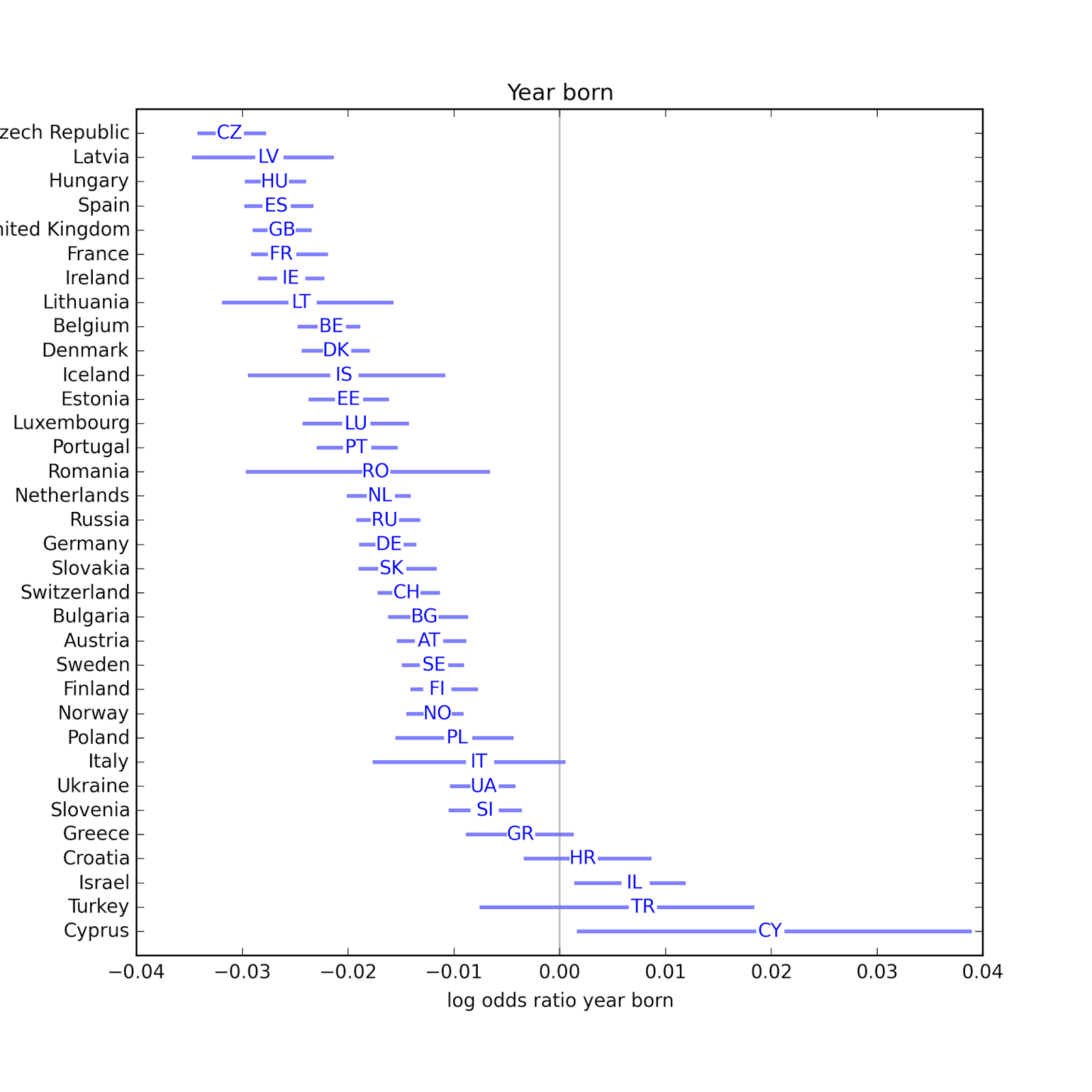 Year born has a consistent negative effect, indicating that younger people are less likely to be affiliated. Possible exceptions are Israel, Turkey and Cyprus.
 In most countries, people with more education are less likely to be affiliated. Possible exceptions: Latvia, Sweden, and the UK.
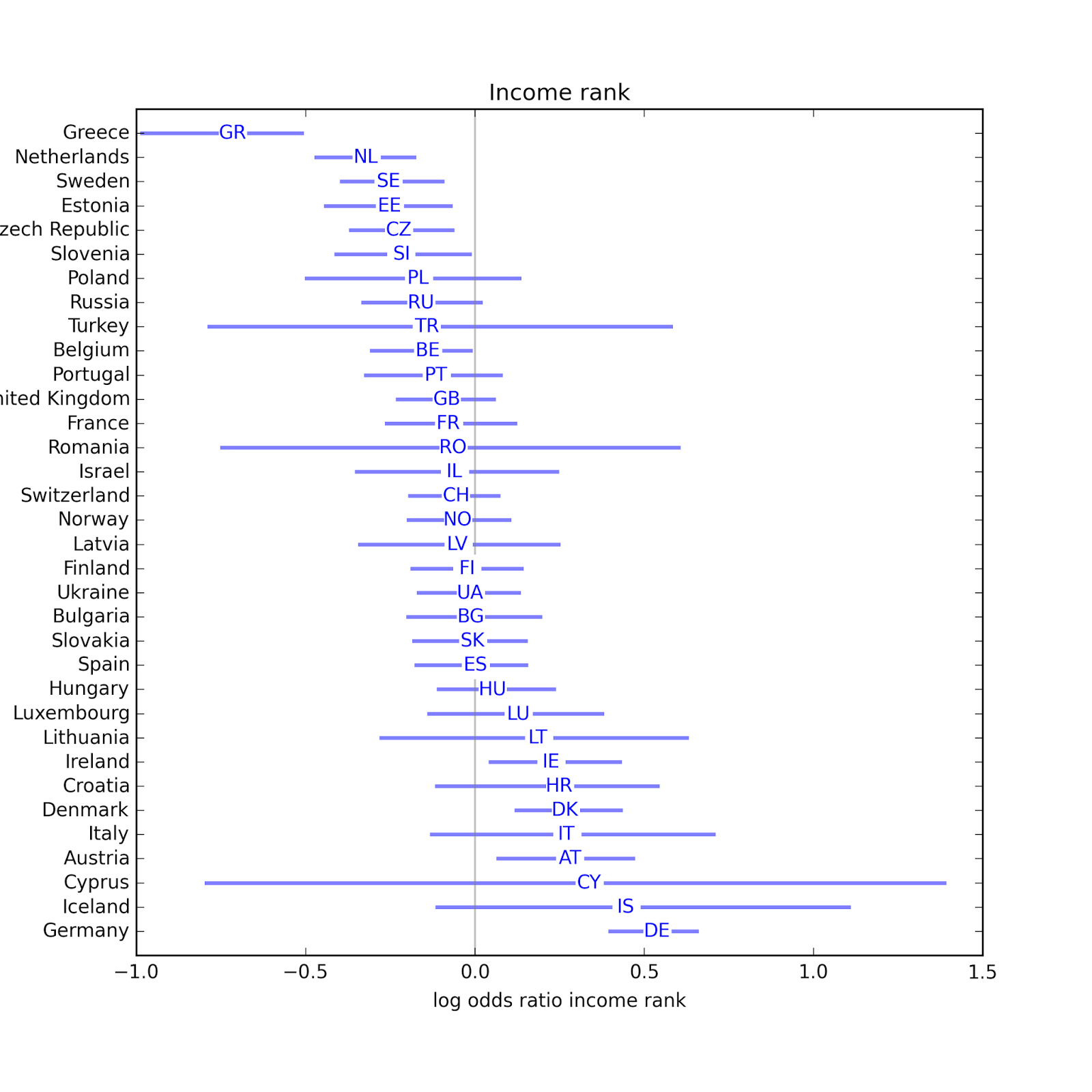 In a few countries, income might have an effect, positive or negative. But it most countries it is not statistically significant.
 It looks like television might have a positive or negative effect in several countries.
 In most countries the effect of radio is not statistically significant. Possible exceptions are Portugal, Greece, Bulgaria, the Netherlands, Estonia, the UK, Belgium, and Germany.
 In most countries the effect of newspapers is not statistically significant. Possible exceptions are Turkey, Greece, Italy, Spain, Croatia, Estonia, Portugal and Norway.
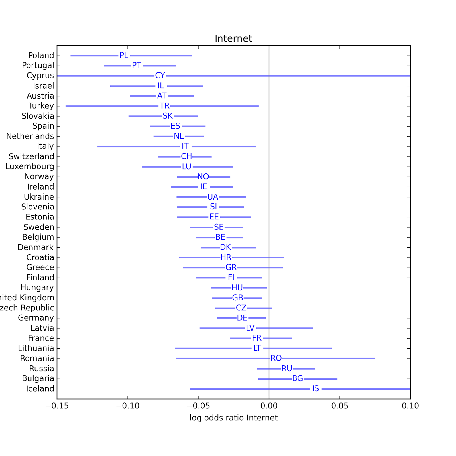 In the majority of countries, Internet use (which includes email and web) is associated with religious disaffiliation. The estimated parameter is only positive in 4 countries, and not statistically significant in any of them. The effect of Internet use appears strongest in Poland, Portugal, Israel, and Austria.
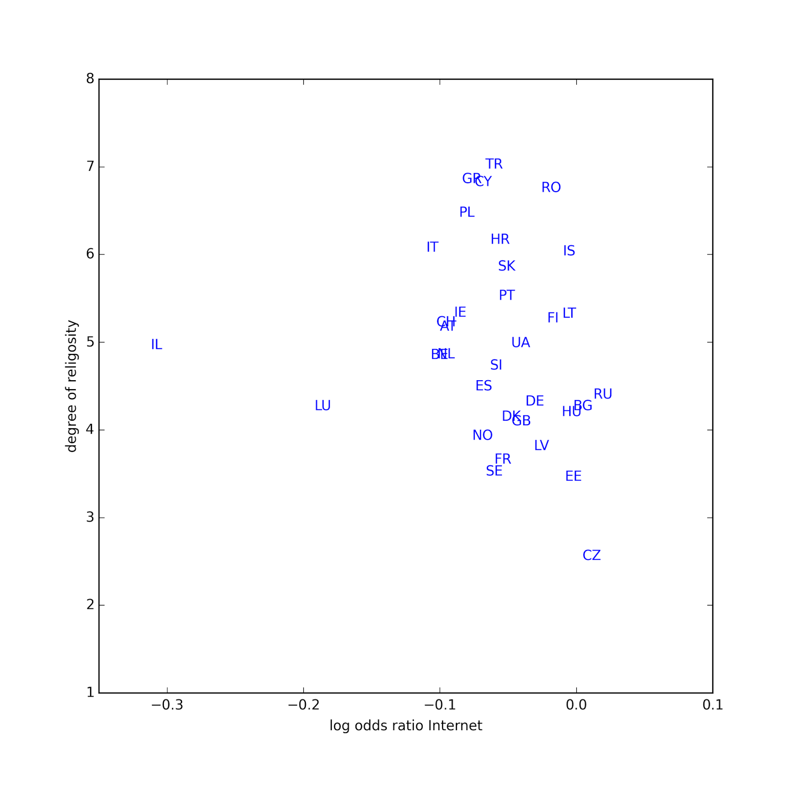
The following scatterplot shows the estimated parameter for Internet use on the x-axis, and the fraction of people who report religious affiliation on the y-axis. There is a weak negative correlation between then (rho = -0.38), indicating that the effect of Internet use is stronger in countries with higher rates of affiliation.

Model 2: Degree of religiosityIn the first model, the dependent variable is rlgdgr, a self-reported degree of religiosity on a 0-10 scale (where 0 = not at all religious and 10 = very religious).
The following figures shows estimated parameters from linear regression, for each of the explanatory variables. Negative values indicate that the variable decreases the likelihood of affiliation; positive values indicate that it increases the likelihood.
Again, the horizontal lines show the 95% confidence interval for the parameters; intervals that cross the zero line are not statistically significant at the p<0.05 level.
 As in Model 1, interview year is almost never statistically significant.
 Younger people are less religious in every country except Israel.
 In most countries, people with more education are less religious, with possible exceptions Estonia, the UK, and Latvia.
 In about half of the countries, people with higher income are less religious. One possible exception: Germany.
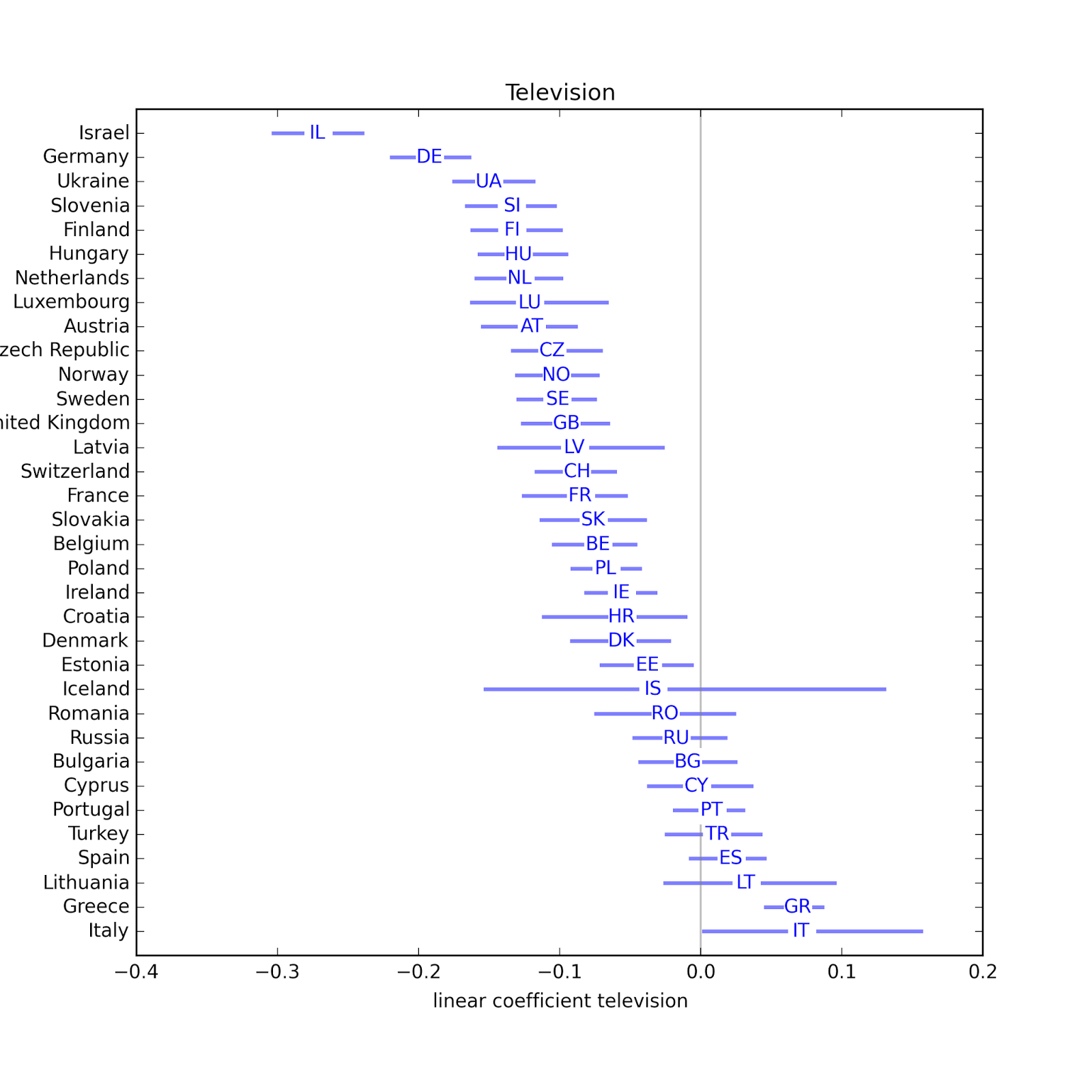 In most countries, people who watch more television are less religious. Possible exceptions: Greece and Italy.
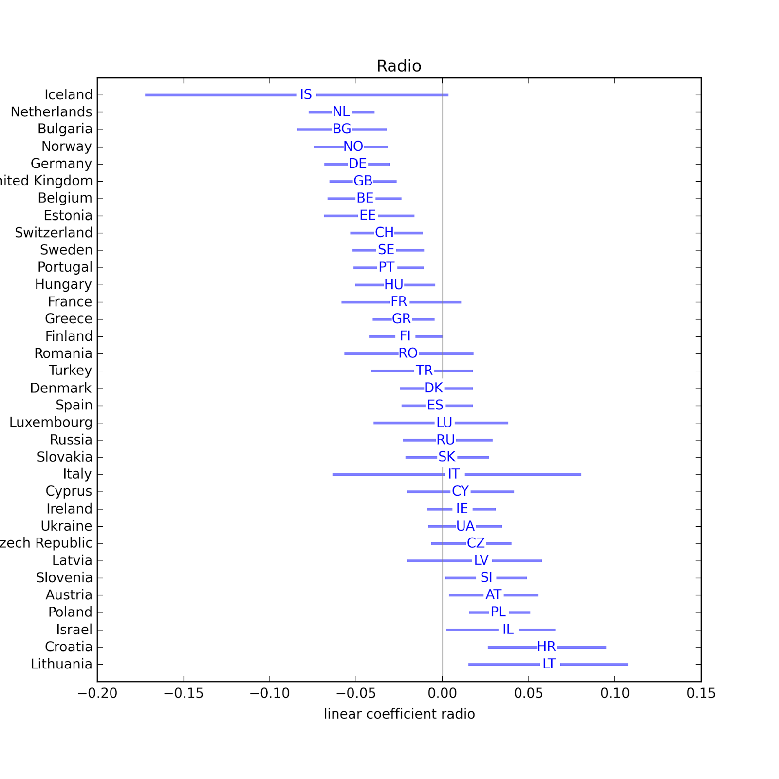 In several countries, people who listen to the radio are less religious. Possible exceptions: Slovenia, Austria, Polans, Israel, Croatia, Lithuania.
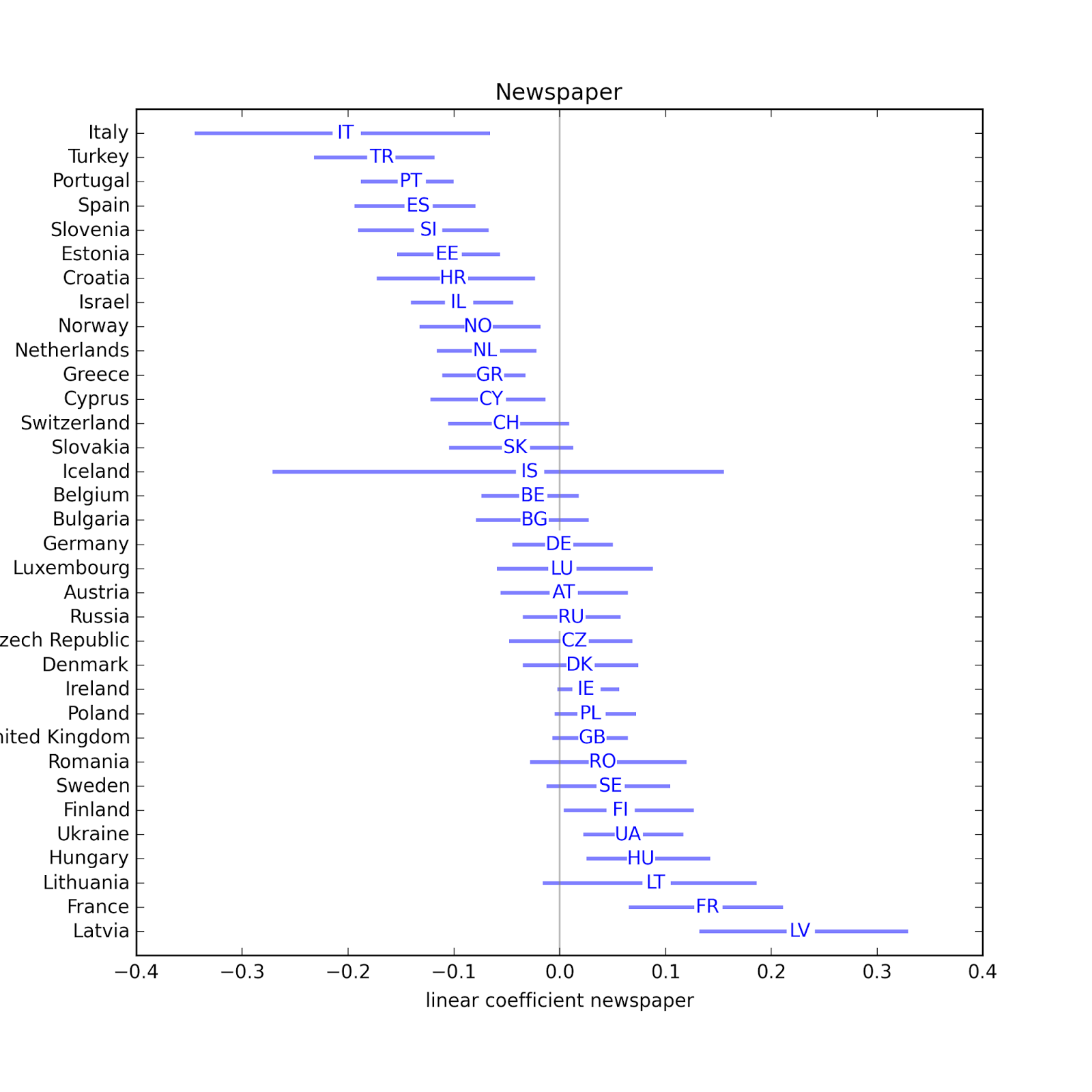 In some countries, people who read newspapers more are less religious, but in some other countries they are more religious.
 In almost every country, people who use the Internet more are less religious. The estimated parameter is only positive in three countries, and none of them are statistically significant. The effect of Internet use appears to be particularly strong in Israel and Luxembourg.
The following scatterplot shows the estimated parameter for Internet use on the x-axis and the national average degree of religiosity on the y-axis. Using all data points, the coefficient of correlation is -0.16, but if we exclude the outliers, it is -0.36, indicating that the effect of Internet use is stronger in countries with higher degrees of religiosity.
 Next stepsI am working on a second round of visualizations that show the size of the Internet effect in each country, expressed in terms of differences between people at the 25th, 50th, and 75th percentiles of Internet use.
I am also open to suggestions for further explorations. And if anyone has insight into some of the countries that show up as exceptions to the common patterns, I would be interested to hear it.

November 17, 2015
Internet use and religion, part two
Cleaning and resamplingHere are the steps of the data cleaning pipeline:
I replace sentinel values with NaNs.I recode some of the explanatory variables, and shift "year born" and "interview year" so their mean is 0.Within each data collection round and each country, I resample the respondents using their post stratification weights (pspwght). In Rounds 1 and 2, there are a few countries that were not asked about Internet use. I remove these countries from those rounds.For the variables eduyrs and hinctnta, I replace each value with its rank (from 0-1) among respondents in the same round and country.I replace missing values with random samples from the same round and country.Finally, I merge rounds 1-5 into a single DataFrame and then group by country.This IPython notebook has the details, and summaries of the variables after processing.
One other difference compared to the previous notebook/article: I've added the variable invyr70, which is the year the respondent was interviewed (between 2002 and 2012), shifted by 2007 so the mean is near 0.
Aggregate resultsUsing variables with missing values filled (as indicated by the _f suffix), I get the following results from logistic regression on rlgblg_f (belonging to a religion), with sample size 233,856:
coefstd errzP>|z|[95.0% Conf. Int.]Intercept1.10960.01766.3810.0001.077 1.142inwyr07_f0.04770.00230.7820.0000.045 0.051yrbrn60_f-0.00900.000-32.6820.000-0.010 -0.008edurank_f0.01320.0170.7750.438-0.020 0.046hincrank_f0.07870.0164.9500.0000.048 0.110tvtot_f-0.01760.002-7.8880.000-0.022 -0.013rdtot_f-0.01300.002-7.7100.000-0.016 -0.010nwsptot_f-0.03560.004-9.9860.000-0.043 -0.029netuse_f-0.10820.002-61.5710.000-0.112 -0.105
Compared to the results from last time, there are a few changesInterview year has a substantial effect, but probably should not be taken too seriously in this model, since the set of countries included in each round varies. The apparent effect of time might reflect the changing mix of countries. I expect this variable to be more useful after we group by country.The effect of "year born" is similar to what we saw before. Younger people are less likely to be affiliated.The effect of education, now expressed in relative terms within each country, is no longer statistically significant. The apparent effect we saw before might have been due to variation across countries.The effect of income, now expressed in relative terms within each country, is now positive, which is more consistent with results in other studies. Again, the apparent negative effect in the previous analysis might have been due to variation across countries (see Simpson's paradox).The effect of the media variables is similar to what we saw before: Internet use has the strongest effect, 2-3 times bigger than newspapers, which are 2-3 times bigger than television or radio. And all are negative.The inconsistent behavior of education and income as control variables is a minor concern, but I think the symptoms are most likely the result of combining countries, possibly made worse because I am not weighting countries by population, so smaller countries are overrepresented.
Here are the results from linear regression with rlgdgr_f (degree of religiosity) as the dependent variable:
coefstd errtP>|t|[95.0% Conf. Int.]Intercept6.01400.022270.4070.0005.970 6.058inwyr07_f0.02530.00212.0890.0000.021 0.029yrbrn60_f-0.01720.000-46.1210.000-0.018 -0.016edurank_f-0.24290.023-10.5450.000-0.288 -0.198hincrank_f-0.15410.022-7.1280.000-0.196 -0.112tvtot_f-0.07340.003-24.3990.000-0.079 -0.067rdtot_f-0.01990.002-8.7600.000-0.024 -0.015nwsptot_f-0.07620.005-15.6730.000-0.086 -0.067netuse_f-0.13740.002-57.5570.000-0.142 -0.133In this model, all parameters are statistically significant. The effect of the media variables, including Internet use, is similar to what we saw before.
The effect of education and income is negative in this model, but I am not inclined to take it too seriously, again because we are combining countries in a way that doesn't mean much.
Breakdown by countryThe following table shows results for logistic regression, with rlgblg_f as the dependent variable, broken down by country; the columns are country code, number of observations, and the estimated parameter associated with Internet use:
Country Num Coef of code obs. netuse_f------- ---- --------AT 6918 -0.0795 ** BE 8939 -0.0299 ** BG 6064 0.0145 CH 9310 -0.0668 ** CY 3293 -0.229 ** CZ 8790 -0.0364 ** DE 11568 -0.0195 * DK 7684 -0.0406 ** EE 6960 -0.0205 ES 9729 -0.0741 ** FI 7969 -0.0228 FR 5787 -0.0185 GB 11117 -0.0262 ** GR 9759 -0.0245 HR 3133 -0.0375 HU 7806 -0.0175 IE 10472 -0.0276 * IL 7283 -0.0636 ** IS 579 0.0333 IT 1207 -0.107 ** LT 1677 -0.0576 * LU 3187 -0.0789 ** LV 1980 -0.00623 NL 9741 -0.0589 ** NO 8643 -0.0304 ** PL 8917 -0.108 ** PT 10302 -0.103 ** RO 2146 0.00855 RU 7544 0.00437 SE 9201 -0.0374 ** SI 7126 -0.0336 ** SK 6944 -0.0635 ** TR 4272 -0.0857 * UA 7809 -0.0422 **
** p < 0.01, * p < 0.05
In the majority of countries, there is a statistically significant relationship between Internet use and religious affiliation. In all of those countries the relationship is negative, with the magnitude of most coefficients between 0.03 and 0.11 (with one exceptionally large value in Cyprus).
Degree of religiosityAnd here are the results of linear regression, with rlgdgr_f as the dependent variable:
Country Num Coef of code obs. netuse_f------- ---- --------AT 6918 -0.0151 ** BE 8939 -0.0072 ** BG 6064 0.0023 CH 9310 -0.0132 ** CY 3293 -0.00221 ** CZ 8790 -0.005 ** DE 11568 -0.0045 * DK 7684 -0.00909 ** EE 6960 -0.00363 ES 9729 -0.0165 ** FI 7969 -0.00501 FR 5787 -0.00429 GB 11117 -0.0061 ** GR 9759 -0.00362 ** HR 3133 -0.00559 HU 7806 -0.00478 * IE 10472 -0.00412 * IL 7283 -0.00419 ** IS 579 0.00752 IT 1207 -0.0212 ** LT 1677 -0.00746 LU 3187 -0.0152 ** LV 1980 -0.00147 NL 9741 -0.014 ** NO 8643 -0.00721 ** PL 8917 -0.00919 ** PT 10302 -0.0149 ** RO 2146 0.000303 RU 7544 0.00102 SE 9201 -0.00815 ** SI 7126 -0.00835 ** SK 6944 -0.0119 ** TR 4272 -0.00331 ** UA 7809 -0.00947 **
In most countries there is a negative and statistically significant relationship between Internet use and degree of religiosity.
In this model the effect of education is consistent: in most countries it is negative and statistically significant. In the two countries where it is positive, it is not statistically significant.
The effect of income is less consistent: in most countries it is not statistically significant; when it is, it is positive as often as negative.
But education and income are in the model primarily as control variables; they are not the focus on this study. If they are actually associated with religious affiliation, these variables should be effective controls; if not, they contribute some noise, but otherwise do no harm.
Next stepsFor now I am using StatsModels to estimate parameters and compute confidence intervals, but that's not quite right because I am using resampled data and filling missing values with random samples. To account correctly for these sources of random error, I have to run the whole process repeatedly:Resample the data.Fill missing values.Estimate parameters.Collecting the estimated parameters from multiple runs, I can estimate the sampling distribution of the parameters and compute confidence intervals.
Once I have implemented that, I plan to translate the results into a form that is easier to interpret (rather than just estimated coefficients), and generate visualizations to make the results easier to explore.
I would also like to relate the effect of Internet use in each country with the average level of religiosity, to see whether, for example, the effect is bigger in more religious countries.
While I am working on that, I am open to suggestions for additional explorations people might be interested in. You can explore the variables in the ESS using their "Cumulative Data Wizard"; let me know what you find!

November 16, 2015
Internet use and religious affiliation in Europe
Since then, I have been planning to replicate the study using data from the European Social Survey, but I didn't get back to it until a few weeks ago. I was reminded about it because they recently released data from Round 7, conducted in 2014. I am always excited about new data, but in this case it doesn't help me: in Rounds 6 and 7 they did not ask about Internet use.
But they did ask in Rounds 1 through 5, collected between 2002 and 2010. So that's something. I downloaded the data, loaded it into Pandas dataframes, and started cleaning, validating, and doing some preliminary exploration. This IPython notebook shows what the first pass looks like.
In the interest of open, replicable science, I am posting preliminary work here, but at this point we should not take the results too seriously.
Data inventoryThe dependent variables I plan to study are
rlgblg: Do you consider yourself as belonging to any particular religion or denomination?
rlgdgr: Regardless of whether you belong to a particular religion, how religious would you say you are?
The explanatory variables are
yrbrn: And in what year were you born?
hinctnta: Using this card, please tell me which letter describes your household's total income, after tax and compulsory deductions, from all sources? If you don't know the exact figure, please give an estimate. Use the part of the card that you know best: weekly, monthly or annual income.
eduyrs: About how many years of education have you completed, whether full-time or part-time? Please report these in full-time equivalents and include compulsory years of schooling.
tvtot: On an average weekday, how much time, in total, do you spend watching television?
rdtot: On an average weekday, how much time, in total, do you spend listening to the radio?
nwsptot: On an average weekday, how much time, in total, do you spend reading the newspapers?
netuse: Now, using this card, how often do you use the internet, the World Wide Web or e-mail - whether at home or at work - for your personal use?
RecodesIncome: I created a variable, hinctnta5, which subtracts 5 from hinctnta, so the mean is near 0. This shift makes the parameters of the model easier to interpret.
Year born: Similarly, I created yrbrn60, which subtracts 1960 from yrbrn.
Years of education: The distribution of eduyrs includes some large values that might be errors, and the question was posed differently in the first few rounds. I will investigate more carefully later, but for now I am replacing values greater than 25 years with 25, and subtracting off the mean, 12, to create eduyrs12.
ResultsJust to get a quick look at things, I ran a logistic regression with rlgblg as the dependent variable, using data Rounds 1-5 and including all countries. The sample size is 229,307. Here are the estimated parameters (computed by StatsModels):
coefstd errzP>|z|[95.0% Conf. Int.]Intercept0.98110.01470.0140.0000.954 1.009yrbrn60-0.00780.000-27.8260.000-0.008 -0.007eduyrs12-0.03760.001-29.6190.000-0.040 -0.035hinctnta5-0.02200.002-12.9340.000-0.025 -0.019tvtot-0.01610.002-7.2050.000-0.021 -0.012rdtot-0.01490.002-8.8260.000-0.018 -0.012nwsptot-0.03200.004-8.9240.000-0.039 -0.025netuse-0.07580.002-42.0620.000-0.079 -0.072
The parameters are all statistically significant with very small p-values. And they are all negative, which indicates:
Younger people are less likely to report a religious affiliation.More educated people are less likely...People with higher income are less likely...People who consume more media (television, radio, newspaper) are less likely...People who use the Internet more are less likely...The effect of Internet use (per hour per week) appears to be about twice the effect of reading the newspaper, which is about twice the effect of television or radio.
The effect of the Internet is comparable to about a decade of age, two years of education, or 3 deciles of income.
Most of these results are consistent with what I saw in my previous study and what other studies have shown. One exception is income: in other studies, the usual pattern is that people in the lowest income groups are less likely to be affiliated, and after that, income has no effect. We'll see if this preliminary result holds up.
I ran a similar model using rlgdgr (degree of religiosity) as the dependent variable:
coefstd errtP>|t|[95.0% Conf. Int.]Intercept5.66680.019300.0710.0005.630 5.704yrbrn60-0.01800.000-47.3520.000-0.019 -0.017eduyrs12-0.06880.002-40.1590.000-0.072 -0.065hinctnta5-0.02660.002-11.3970.000-0.031 -0.022tvtot-0.08010.003-26.3340.000-0.086 -0.074rdtot-0.01790.002-7.7910.000-0.022 -0.013nwsptot-0.05310.005-10.8730.000-0.063 -0.044netuse-0.10200.002-40.9420.000-0.107 -0.097
The results are similar. Again, this IPython notebook has the details.
LimitationsAgain, we should not take these results too seriously yet:
So far I am not taking into account the weights associated with respondents, either within or across countries. So for now I am oversampling people in small countries, as well as some groups within countries.At this point I haven't done anything careful to fill missing values, so the results will change when I get that done.And I think it will be more meaningful to break the results down by country.Stay tuned. More coming soon!

November 13, 2015
Recidivism and logistic regression
My collaborator asked me to compare two methods and explain their assumptions, properties, pros and cons:
1) Logistic regression: This is the standard method in the field. Researchers have designed a survey instrument that assigns each offender a score from -3 to 12. Using data from previous offenders, they estimate the parameters of a logistic regression model and generate a predicted probability of recidivism for each score.
2) Post test probabilities: An alternative of interest to my collaborator is the idea of treating survey scores the way some tests are used in medicine, with a threshold that distinguishes positive and negative results. Then for people who "test positive" we can compute the post-test probability of recidivism.
In addition to these two approaches, I considered three other models:
3) Independent estimates for each group: In the previous article, I cited the notion that "the probability of recidivism for an individual offender will be the same as the observed recidivism rate for the group to which he most closely belongs." (Harris and Hanson 2004). If we take this idea to an extreme, the estimate for each individual should be based only on observations of the same risk group. The logistic regression model is holistic in the sense that observations from each group influence the estimates for all groups. An individual who scores a 6, for example, might reasonably object if the inclusion of offenders from other risk classes has the effect of increasing the estimated scores for his own class. To evaluate this concern, I also considered a simple model where the risk in each group is estimated independently.
4) Logistic regression with a quadratic term: Simple logistic regression is based on the assumption that the scores are linear in the sense that each increment corresponds to the same increase in risk; for example, it assumes that the odds ratio between groups 1 and 2 is the same as the odds ratio between groups 9 and 10. To test that assumption, I ran a model that includes the square of the scores as a predictive variable. If risks are actually non-linear, this quadratic term might provide a better fit to the data. But it doesn't, so the linear assumption holds up, at least to this simple test.
5) Bayesian logistic regression: This is a natural extension of logistic regression that takes as inputs prior distributions for the parameters, and generates posterior distributions for the parameters and predictive distributions for the risks in each group. For this application, I didn't expect this approach to provide any great advantage over conventional logistic regression, but I think the Bayesian version is a powerful and surprisingly simple idea, so I used this project as an excuse to explore it.
Details of these methods are in this IPython notebook; I summarize the results below.
Logistic regressionMy collaborator provided a dataset with 10-year recidivism outcomes for 703 offenders. The definition of recidivism in this case is that the individual was charged with another offense within 10 years of release (but not necessarily convicted). The range of scores for offenders in the dataset is from -2 to 11.
I estimated parameters using the StatsModels module. The following figure shows the estimated probability of recidivism for each score and the predictive 95% confidence interval.
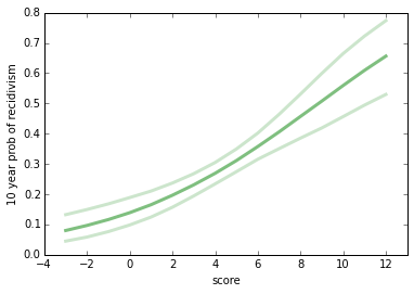
A striking feature of this graph is the range of risks, from less than 10% to more than 60%. This range suggests that it is important to get this right, both for the individuals involved and for society.
[One note: the logistic regression model is linear when expressed in log-odds, so it is not a straight line when expressed in probabilities.]
Post test probabilitiesIn the context of medical testing, a "post-test probability/positive" (PTPP) is the answer to the question, "Given that a patient has tested positive for a condition of interest (COI), what is the probability that the patient actually has the condition, as opposed to a false positive test". The advantage of PTPP in medicine is that it addresses the question that is arguably most relevant to the patient.
In the context of recidivism, if we want to treat risk scores as a binary test, we have to choose a threshold that splits the range into low and high risk groups. As an example, if I choose "6 or more" as the threshold, I can compute the test's sensitivity, specificity, and PTPP:
With threshold 6, the sensitivity of the test is 42%, meaning that the test successfully identifies (or predicts) 42% of recidivists.The specificity is 76%, which is the fraction of non-recidivists who correctly test negative.The PTPP is 42%, meaning that 42% of the people who test positive will reoffend. [Note: it is only a coincidence in this case that sensitivity and PTPP are approximately equal.]One of the questions my collaborator asked is whether it's possible to extend this analysis to generate a posterior distribution for PTPP, rather than a point estimate. In the notebook I show how to do that using beta distributions for the priors and posteriors. For this example, the 95% posterior credible interval is 35% to 49%.
Now suppose we customize the test for each individual. So if someone scores 3, we would set the threshold to 3 and compute a PTPP and a credible interval. We could treat the result as the probability of recidivism for people who test 3 or higher. The following figure shows the results (in blue) superimposed on the results from logistic regression (in grey).

A few features are immediately apparent:
At the low end of the range, PTPP is substantially higher than the risk estimated by logistic regression.At the high end, PTPP is lower.With this dataset, it's not possible to compute PTPP for the lowest and highest scores (as contrasted with logistic regression, which can extrapolate).For the lowest risk scores, the credible intervals on PTPP are a little smaller than the confidence intervals of logistic regression.For the high risk scores, the credible intervals are very large, due to the small amount of data.So there are practical challenges in estimating PTPPs with a small dataset. There are also philosophical challenges. If the goal is to estimate the risk of recidivism for an individual, it's not clear that PTPP is the answer to the right question.
This way of using PTPP has the effect of putting each individual in a reference class with everyone who scored the same or higher. Someone who is subject to this test could reasonably object to being lumped with higher-risk offenders. And they might reasonably ask why it's not the other way around: why is the reference class "my risk or higher" and not "my risk or lower"?
I'm not sure there is a principled reason to that question. In general, we should prefer a smaller reference class, and one that does not systematically bias the estimates. Using PTPP (as proposed) doesn't do well by these criteria.
But logistic regression is vulnerable to the same objection: outcomes from high-risk offenders have some effect on the estimates for lower-risk groups. Is that fair?
Independent estimatesTo answer that question, I also ran a simple model that estimates the risk for each score independently. I used a uniform distribution as a prior for each group, computed a Bayesian posterior distribution, and plotted the estimated risks and credible intervals. Here are the results, again superimposed on the logistic regression model.

People who score 0, 1, or 8 or more would like this model. People who score -2, 2, or 7 would hate it. But given the size of the credible intervals, it's clear that we shouldn't take these variations too seriously.
With a bigger dataset, the credible intervals would be smaller, and we expect the results to be ordered so that groups with higher scores have higher rates of recidivism. But with this small dataset, we have some practical problems.
We could smooth the data by combining adjacent scores into risk ranges. But then we're faced again with the objection that this kind of lumping is unfair to people at the low end of each range, and dangerously generous to people at the high end.
I think logistic regression balances these conflicting criteria reasonably: by taking advantage of background information -- the assumption that higher scores correspond to higher risks -- it uses data efficiently, generating sensible estimates for all scores and confidence intervals that represent the precision of the estimates.
However, it is based on an assumption that might be too strong, that the relationship between log-odds and risk score is linear. If that's not true, the model might be unfair to some groups and too generous to others.
Linear regression with a quadratic termTo see whether the linear assumption is valid, we can run logistic regression again with two explanatory variables: score and the square of score. If the relationship is actually non-linear, this quadratic model might fit the data better.
The estimated coefficient for the quadratic term is negative, so the line of best fit is a parabola with downward curvature. That's consistent with the shape of the independent estimates in the previous section. But the estimate for the quadratic parameter is not statistically significant (p=0.11), which suggests that it might be due to randomness.
Here is what the results look like graphically, again compared to the logistic regression model:

The estimates are lower for the lowest score groups, about the same in the middle, and lower again for the highest scores. At the high end, it seems unlikely that the risk of recidivism actually declines for the highest scores, and more likely that we are overfitting the data.
This model suggests that the linear logistic regression might overestimate risk for the lowest-scoring groups. It might be worth exploring this possibility with more data.
Bayesian logistic regressionOne of the best features of logistic regression is that the results are in the form of a probability, which is useful for all kinds of analysis and especially for the kind of risk-benefit analysis that underlies parole decisions.
But conventional logistic regression does not admit prior information about the parameters, and the result is not a posterior distribution, but just a point estimate and confidence interval. In general, confidence intervals are less useful as part of a decision making process. And if you have ever tried to explain a confidence interval to a general audience, you know they can be problematic.
So, mostly for my own interest, I applied Bayesian logistic regression to the same data. The Bayesian version of logistic regression is conceptually simple and easy to implement, in part because at the core of logistic regression there is a tight connection to Bayes's theorem. I wrote about this connection in a previous article.
My implementation, with explanatory comments, is in the IPython notebook; here are the results:
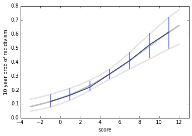
With a uniform prior for the parameters, the results are almost identical to the results from (conventional) logistic regression. At first glance it seems like the Bayesian version has no advantage, but there are a few reasons it might:
For each score, we can generate a posterior distribution that represents not just a point estimate, but all possible estimates and their probabilities. If the posterior mean is 55%, for example, we might want to know the probability that the correct value is more than 65%, or less than 45%. The posterior distribution can answer this question; conventional logistic regression cannot.If we use estimates from the model as part of another analysis, we could carry the posterior distribution through the subsequent computation, producing a posterior predictive distribution for whatever results the analysis generates.If we have background information that guides the choice of the prior distributions, we could use that information to produce better estimates.But in this example, I don't have a compelling reason to choose a different prior, and there is no obvious need for a posterior distribution: a point estimate is sufficient. So (although it hurts me to admit it) the Bayesian version of logistic regression has no practical advantage for this application.
SummaryUsing logistic regression to estimate the risk of recidivism for each score group makes good use of the data and background information. Although the estimate for each group is influenced by outcomes in other groups, this influence is not unfair in any obvious way.
The alternatives I considered are problematic: PTPP is vulnerable to both practical and philosophical objections. Estimating risks for each group independently is impractical with a small dataset, but might work well with more data.
The quadratic logistic model provides no apparent benefit, and probably overfits the data. The Bayesian version of logistic regression is consistent with the conventional version, and has no obvious advantages for this application.

Probably Overthinking It

- Allen B. Downey's profile
- 236 followers

