
Allen B. Downey's Blog: Probably Overthinking It, page 21
November 9, 2015
Recidivism and single-case probabilities
I am collaborating with a criminologist who studies recidivism. In the context of crime statistics, a recidivist is a convicted criminal who commits a new crime post conviction. Statistical studies of recidivism are used in parole hearings to assess the risks of releasing a prisoner. This application of statistics raises questions that go to the foundations of probability theory.
Specifically, assessing risk for an individual is an example of a "single-case probability", a well-known problem in the philosophy of probability. For example, we would like to be able to make a statement like, "If released, there is a 55% probability that Mr. Smith will be charged with another crime within 10 years." But how could we estimate a probability like that, and what would it mean?
I suggest we answer these questions in three steps. The first is to choose a "reference class"; the second is to estimate the probability of recidivism in the reference class; the third is to interpret the result as it applies to Mr. Smith.
For example, if the reference class includes all people convicted of the same crime as Mr. Smith, we could find a sample of that population and compute the rate of recidivism in the sample. If 55% of the sample were recidivists, we might claim that Mr. Smith has a 55% probability of reoffending.
Let's look at those steps in more detail:
1) The reference class problem For any individual offender, there are an unbounded number of reference classes we might choose. For example, if we consider characteristics like age, marital status, and severity of crime, we might form a reference class using any one of those characteristics, any two, or all three. As the number of characteristics increases, the number of possible classes grows exponentially (and I mean that literally, not as a sloppy metaphor for "very fast").
Some reference classes are preferable to others; in general, we would like the people in each class to be as similar as possible to each other, and the classes to be as different as possible from each other. But there is no objective procedure for choosing the "right" reference class.
2) Sampling and estimation Assuming we have chosen a reference class, we would like to estimate the proportion of recidivists in the class. First, we have to define recidivism in a way that's measurable. Ideally we would like to know whether each member of the class commits another crime, but that's not possible. Instead, recidivism is usually defined to mean that the person is either charged or convicted of another crime.
If we could enumerate the members of class and count recidivists and non-, we would know the true proportion, but normally we can't do that. Instead we choose a sampling process intended to select a representative sample, meaning that every member of the class has the same probability of appearing in the sample, and then use the observed proportion in the sample to estimate the true proportion in the class.
3) Interpretation Suppose we agree on a reference class, C, a sampling process, and an estimation process, and estimate that the true proportion of recidivists in C is 55%. What can we say about Mr. Smith?
As my collaborator has demonstrated, this question is a topic of ongoing debate. Among practitioners in the field, some take the position that "the probability of recidivism for an individual offender will be the same as the observed recidivism rate for the group to which he most closely belongs." (Harris and Hanson 2004). On this view, we would conclude that Mr. Smith has a 55% chance of reoffending.
Others take the position that this claim is nonsense because it could never be confirmed or denied; whether Mr. Smith goes on to commit another crime or not, neither outcome supports or refutes the claim that the probability was 55%. On this view, probability cannot be meaningfully applied to a single event.
To understand this view, consider an analogy suggested by my colleague Rehana Patel: Suppose you estimate that the median height of people in class C is six feet. You could not meaningfully say that the median height of Mr. Smith is six feet. Only the class has a median height, individuals do not. Similarly, only the class has a proportion of recidivists; individuals do not.
And the answer is...At this point I have framed the problem and tried to state the opposing views clearly. Now I will explain my own view and try to justify it.
I think it is both meaningful and useful to say, in the example, that Mr. Smith has a 55% chance of offending again. Contrary to the view that no possible outcome supports or refutes this claim, Bayes's theorem tells us otherwise. Suppose we consider two hypotheses:
H55: Mr. Smith has a 55% chance of reoffending.
H45: Mr. Smith has a 45% chance of reoffending.
If Mr. Smith does in fact commit another crime, this datum supports H55 with a Bayes factor of (55)/(45) = 1.22. And if he does not, that datum supports H45 by the same factor. In either case it is weak evidence, but nevertheless it is evidence, which means that H55 is a meaningful claim that can be supported or refuted by data. The same argument applies if there are more than two discrete hypotheses or a continuous set of hypotheses.
Furthermore, there is a natural operational interpretation of the claim. If we consider some number, n, of individuals from class C, and estimate that each of them has probability, p, of reoffending, we can compute a predictive distribution for k, the number who reoffend. It is just the binomial distribution of k with parameters p and n:
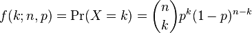
For example, if n=100 and p=55, the most likely value of k is 55, and the probability that k=55 is about 8%. As far as I know, no one has a problem with that conclusion.
But if there is no philosophical problem with the claim, "Of these 100 members of class C, the probability that 55 of them will reoffend is 8%", there should be no special problem when n=1. In that case we would say, "Of these 1 members of class C, the probability that 1 will reoffend is 55%." Granted, that's a funny way to say it, but that's a grammatical problem, not a philosophical one.
Now let me address the challenge of the height analogy. I agree that Mr. Smith does not have a median height; only groups have medians. However, if the median height in C is six feet, I think it is correct to say that Mr. Smith has a 50% chance of being taller than six feet.
That might sound strange; you might reply, "Mr. Smith's height is a deterministic physical quantity. If we measure it repeatedly, the result is either taller than six feet every time, or shorter every time. It is not a random quantity, so you can't talk about its probability."
I think that reply is mistaken, because it leaves out a crucial step:
1) If we choose a random member of C and measure his height, the result is a random quantity, and the probability that it exceeds six feet is 50%.
2) We can consider Mr. Smith to be a randomly-chosen member of C, because part of the notion of a reference class is that we consider the members to be interchangeable.
3) Therefore Mr. Smith's height is a random quantity and we can make probabilistic claims about it.
My use of the word "consider" in the second step is meant to highlight that this step is a modeling decision: if we choose to regard Mr. Smith as a random selection from C, we can treat his characteristics as random variables. The decision not to distinguish among the members of the class is part of what it means to choose a reference class.
Finally, if the proportion of recidivists in C is 55%, the probability that a random member of C will reoffend is 55%. If we consider Mr. Smith to be a random member of C, his probability of reoffending is 55%.
Is this useful?I have argued that it is meaningful to claim that Mr. Smith has a 55% probability of recidivism, and addressed some of the challenges to that position.
I also think that claims like this are useful because they guide decision making under uncertainty. For example, if Mr. Smith is being considered for parole, we have to balance the costs and harms of keeping him in prison with the possible costs and harms of releasing him. It is probably not possible to quantify all of the factors that should be taken into consideration in this decision, but it seems clear that the probability of recidivism is an important factor.
Furthermore, this probability is most useful if expressed in absolute, as opposed to relative, terms. If we know that one prisoner has a higher risk than another, that provides almost no guidance about whether either should be released. But if one has a probability of 10% and another 55% (and those are realistic numbers for some crimes) those values could be used as part of a risk-benefit analysis, which would usefully inform individual decisions, and systematically yield better outcomes.
What about the Bayesians and the Frequentists?When I started this article, I thought the central issue was going to be the difference between the Frequentist and Bayesian interpretations of probability. But I came to the conclusion that this distinction is mostly irrelevant.
Considering the three steps of the process again:
1) Reference class: Choosing a reference class is equally problematic under either interpretation of probability; there is no objective process that identifies the right, or best, reference class. The choice is subjective, but that is not to say arbitrary. There are reasons to prefer one model over another, but because there are multiple relevant criteria, there is no unique best choice.
2) Estimation: The estimation step can be done using frequentist or Bayesian methods, and there are reasons to prefer one or the other. Some people argue that Bayesian methods are more subjective because they depend on a prior distribution, but I think both approaches are equally subjective; the only difference is whether the priors are explicit. Regardless, the method you use to estimate the proportion of recidivists in the reference class has no bearing on the third step.
3) Interpretation: In my defense of the claim that the proportion of recidivists in the reference class is the probability of recidivism for the individual, I used Bayes's theorem, which is a universally accepted law of probability, but I did not invoke any particular interpretation of probability.
I argued that we could treat an unknown quantity as a random variable. That idea is entirely unproblematic under Bayesianism, but less obviously compatible with frequentism. Some sources claim that frequentism is specifically incompatible with single-case probabilities.
For example the Wikipedia article on probability interpretations claims that "Frequentists are unable to take this approach [a propensity interpretation], since relative frequencies do not exist for single tosses of a coin, but only for large ensembles or collectives."
I don't agree that assigning a probability to a single case is a special problem for frequentism. Single case probabilities seem hard because they make the choice of the reference class more difficult. But choosing a reference class is hard under any interpretation of probability; it is not a special problem for frequentism.
And once you have chosen a reference class, you can estimate parameters of the class and generate predictions for individuals, or groups, without commitment to a particular interpretation of probability.
[For more about alternative interpretations of probability, and how they handle single-case probabilities, see this article in the Stanford Encyclopedia of Philosophy, especially the section on frequency interpretations. As I read it, the author agrees with me that (1) the problem of the single case relates to choosing a reference class, not attributing probabilities to individuals, and (2) in choosing a reference class, there is no special problem with the single case that is not also a problem in other cases. If there is any difference, it is one of degree, not kind.]
Summary
In summary, the assignment of a probability to an individual depends on three subjective choices:
1) The reference class,
2) The prior used for estimation,
3) The modeling decision to regard an individual as a random sample with n=1.
You can think of (3) as an additional choice or as part of the definition of the reference class.
These choices are subjective but not arbitrary; that is, there are justified reasons to prefer one over others, and to accept some as good enough for practical purposes.
Finally, subject to those choices, it is meaningful and useful to make claims like "Mr. Smith has a 55% probability of recidivism".
Q&A
1) Isn't it dehumanizing to treat an individual as if he were an interchangeable, identical member of a reference class? Every human is unique; you can't treat a person like a number!
I conjecture that everyone who applies quantitative methods to human endeavors has heard a complaint like this. If the intended point is, "You should never apply quantitative models to humans," I disagree. Everything we know about the world, including the people in it, is mediated by models, and all models are based on simplifications. You have to decide what to include and what to leave out. If your model includes the factors that matter and omits the ones that don't, it will be useful for practical purposes. If you make bad modeling decisions, it won't.
But if the intent of this question is to say, "Think carefully about your modeling decisions, validate your models as much as practically possible, and consider the consequences of getting it wrong," then I completely agree.
Model selection has consequences. If we fail to include a relevant factor (that is, one that has predictive power), we will treat some individuals unfairly and systematically make decisions that are less good for society. If we include factors that are not predictive, our predictions will be more random and possibly less fair.
And those are not the only criteria. For example, if it turns out that a factor, like race, has predictive power, we might choose to exclude it from the model anyway, possibly decreasing accuracy in order to avoid a particularly unacceptable kind of injustice.
So yes, we should think carefully about model selection, but no, we should not exclude humans from the domain of statistical modeling.
2) Are you saying that everyone in a reference class has the same probability of recidivism? That can't be true; there must be variation within the group.
I'm saying that an individual only has a probability AS a member of a reference class (or, for the philosophers, qua a member of a reference class). You can't choose a reference class, estimate the proportion for the class, and then speculate about different probabilities for different members of the class. If you do, you are just re-opening the reference class question.
To make that concrete, suppose there is a standard model of recidivism that includes factors A, B, and C, and excludes factors D, E, and F. And suppose that the model estimates that Mr. Smith's probability of recidivism is 55%.
You might be tempted to think that 55% is the average probability in the group, and the probability for Mr. Smith might be higher or lower. And you might be tempted to adjust the estimate for Mr. Smith based on factor D, E, or F.
But if you do that, you are effectively replacing the standard model with a new model that includes additional factors. In effect, you are saying that you think the standard model leaves out an important factor, and would be better if it included more factors.
That might be true, but it is a question of model selection, and should be resolved by considering model selection criteria.
It is not meaningful or useful to talk about differences in probability among members of a reference class. Part of the definition of reference class is the commitment to treat the members as equivalent.
That commitment is a modeling decision, not a claim about the world. In other words, when we choose a model, we are not saying that we think the model captures everything about the world. On the contrary, we are explicitly acknowledging that it does not. But the claim (or sometimes the hope) is that it captures enough about the world to be useful.
3) What happened to the problem of the single case? Is it a special problem for frequentism? Is it a special problem at all?
There seems to be some confusion about whether the problem of the single case relates to choosing a reference class (my step 1) or attributing a probability to an individual (step 3).
I have argued that it does not relate to step 3. Once you have chosen a reference class and estimated its parameters, there is no special problem in applying the result to the case of n=1, not under frequentism or any other interpretation I am aware of.
During step 1, single case predictions might be more difficult, because the choice of reference class is less obvious or people might be less likely to agree. But there are exceptions of both kinds: for some single cases, there might be an easy consensus on an obvious good reference class; for some non-single cases, there are many choices and no consensus. In all cases, the choice of reference class is subjective, but guided by the criteria of model choice.
So I think the single case problem is just an instance of the reference class problem, and not a special problem at all.

Specifically, assessing risk for an individual is an example of a "single-case probability", a well-known problem in the philosophy of probability. For example, we would like to be able to make a statement like, "If released, there is a 55% probability that Mr. Smith will be charged with another crime within 10 years." But how could we estimate a probability like that, and what would it mean?
I suggest we answer these questions in three steps. The first is to choose a "reference class"; the second is to estimate the probability of recidivism in the reference class; the third is to interpret the result as it applies to Mr. Smith.
For example, if the reference class includes all people convicted of the same crime as Mr. Smith, we could find a sample of that population and compute the rate of recidivism in the sample. If 55% of the sample were recidivists, we might claim that Mr. Smith has a 55% probability of reoffending.
Let's look at those steps in more detail:
1) The reference class problem For any individual offender, there are an unbounded number of reference classes we might choose. For example, if we consider characteristics like age, marital status, and severity of crime, we might form a reference class using any one of those characteristics, any two, or all three. As the number of characteristics increases, the number of possible classes grows exponentially (and I mean that literally, not as a sloppy metaphor for "very fast").
Some reference classes are preferable to others; in general, we would like the people in each class to be as similar as possible to each other, and the classes to be as different as possible from each other. But there is no objective procedure for choosing the "right" reference class.
2) Sampling and estimation Assuming we have chosen a reference class, we would like to estimate the proportion of recidivists in the class. First, we have to define recidivism in a way that's measurable. Ideally we would like to know whether each member of the class commits another crime, but that's not possible. Instead, recidivism is usually defined to mean that the person is either charged or convicted of another crime.
If we could enumerate the members of class and count recidivists and non-, we would know the true proportion, but normally we can't do that. Instead we choose a sampling process intended to select a representative sample, meaning that every member of the class has the same probability of appearing in the sample, and then use the observed proportion in the sample to estimate the true proportion in the class.
3) Interpretation Suppose we agree on a reference class, C, a sampling process, and an estimation process, and estimate that the true proportion of recidivists in C is 55%. What can we say about Mr. Smith?
As my collaborator has demonstrated, this question is a topic of ongoing debate. Among practitioners in the field, some take the position that "the probability of recidivism for an individual offender will be the same as the observed recidivism rate for the group to which he most closely belongs." (Harris and Hanson 2004). On this view, we would conclude that Mr. Smith has a 55% chance of reoffending.
Others take the position that this claim is nonsense because it could never be confirmed or denied; whether Mr. Smith goes on to commit another crime or not, neither outcome supports or refutes the claim that the probability was 55%. On this view, probability cannot be meaningfully applied to a single event.
To understand this view, consider an analogy suggested by my colleague Rehana Patel: Suppose you estimate that the median height of people in class C is six feet. You could not meaningfully say that the median height of Mr. Smith is six feet. Only the class has a median height, individuals do not. Similarly, only the class has a proportion of recidivists; individuals do not.
And the answer is...At this point I have framed the problem and tried to state the opposing views clearly. Now I will explain my own view and try to justify it.
I think it is both meaningful and useful to say, in the example, that Mr. Smith has a 55% chance of offending again. Contrary to the view that no possible outcome supports or refutes this claim, Bayes's theorem tells us otherwise. Suppose we consider two hypotheses:
H55: Mr. Smith has a 55% chance of reoffending.
H45: Mr. Smith has a 45% chance of reoffending.
If Mr. Smith does in fact commit another crime, this datum supports H55 with a Bayes factor of (55)/(45) = 1.22. And if he does not, that datum supports H45 by the same factor. In either case it is weak evidence, but nevertheless it is evidence, which means that H55 is a meaningful claim that can be supported or refuted by data. The same argument applies if there are more than two discrete hypotheses or a continuous set of hypotheses.
Furthermore, there is a natural operational interpretation of the claim. If we consider some number, n, of individuals from class C, and estimate that each of them has probability, p, of reoffending, we can compute a predictive distribution for k, the number who reoffend. It is just the binomial distribution of k with parameters p and n:
For example, if n=100 and p=55, the most likely value of k is 55, and the probability that k=55 is about 8%. As far as I know, no one has a problem with that conclusion.
But if there is no philosophical problem with the claim, "Of these 100 members of class C, the probability that 55 of them will reoffend is 8%", there should be no special problem when n=1. In that case we would say, "Of these 1 members of class C, the probability that 1 will reoffend is 55%." Granted, that's a funny way to say it, but that's a grammatical problem, not a philosophical one.
Now let me address the challenge of the height analogy. I agree that Mr. Smith does not have a median height; only groups have medians. However, if the median height in C is six feet, I think it is correct to say that Mr. Smith has a 50% chance of being taller than six feet.
That might sound strange; you might reply, "Mr. Smith's height is a deterministic physical quantity. If we measure it repeatedly, the result is either taller than six feet every time, or shorter every time. It is not a random quantity, so you can't talk about its probability."
I think that reply is mistaken, because it leaves out a crucial step:
1) If we choose a random member of C and measure his height, the result is a random quantity, and the probability that it exceeds six feet is 50%.
2) We can consider Mr. Smith to be a randomly-chosen member of C, because part of the notion of a reference class is that we consider the members to be interchangeable.
3) Therefore Mr. Smith's height is a random quantity and we can make probabilistic claims about it.
My use of the word "consider" in the second step is meant to highlight that this step is a modeling decision: if we choose to regard Mr. Smith as a random selection from C, we can treat his characteristics as random variables. The decision not to distinguish among the members of the class is part of what it means to choose a reference class.
Finally, if the proportion of recidivists in C is 55%, the probability that a random member of C will reoffend is 55%. If we consider Mr. Smith to be a random member of C, his probability of reoffending is 55%.
Is this useful?I have argued that it is meaningful to claim that Mr. Smith has a 55% probability of recidivism, and addressed some of the challenges to that position.
I also think that claims like this are useful because they guide decision making under uncertainty. For example, if Mr. Smith is being considered for parole, we have to balance the costs and harms of keeping him in prison with the possible costs and harms of releasing him. It is probably not possible to quantify all of the factors that should be taken into consideration in this decision, but it seems clear that the probability of recidivism is an important factor.
Furthermore, this probability is most useful if expressed in absolute, as opposed to relative, terms. If we know that one prisoner has a higher risk than another, that provides almost no guidance about whether either should be released. But if one has a probability of 10% and another 55% (and those are realistic numbers for some crimes) those values could be used as part of a risk-benefit analysis, which would usefully inform individual decisions, and systematically yield better outcomes.
What about the Bayesians and the Frequentists?When I started this article, I thought the central issue was going to be the difference between the Frequentist and Bayesian interpretations of probability. But I came to the conclusion that this distinction is mostly irrelevant.
Considering the three steps of the process again:
1) Reference class: Choosing a reference class is equally problematic under either interpretation of probability; there is no objective process that identifies the right, or best, reference class. The choice is subjective, but that is not to say arbitrary. There are reasons to prefer one model over another, but because there are multiple relevant criteria, there is no unique best choice.
2) Estimation: The estimation step can be done using frequentist or Bayesian methods, and there are reasons to prefer one or the other. Some people argue that Bayesian methods are more subjective because they depend on a prior distribution, but I think both approaches are equally subjective; the only difference is whether the priors are explicit. Regardless, the method you use to estimate the proportion of recidivists in the reference class has no bearing on the third step.
3) Interpretation: In my defense of the claim that the proportion of recidivists in the reference class is the probability of recidivism for the individual, I used Bayes's theorem, which is a universally accepted law of probability, but I did not invoke any particular interpretation of probability.
I argued that we could treat an unknown quantity as a random variable. That idea is entirely unproblematic under Bayesianism, but less obviously compatible with frequentism. Some sources claim that frequentism is specifically incompatible with single-case probabilities.
For example the Wikipedia article on probability interpretations claims that "Frequentists are unable to take this approach [a propensity interpretation], since relative frequencies do not exist for single tosses of a coin, but only for large ensembles or collectives."
I don't agree that assigning a probability to a single case is a special problem for frequentism. Single case probabilities seem hard because they make the choice of the reference class more difficult. But choosing a reference class is hard under any interpretation of probability; it is not a special problem for frequentism.
And once you have chosen a reference class, you can estimate parameters of the class and generate predictions for individuals, or groups, without commitment to a particular interpretation of probability.
[For more about alternative interpretations of probability, and how they handle single-case probabilities, see this article in the Stanford Encyclopedia of Philosophy, especially the section on frequency interpretations. As I read it, the author agrees with me that (1) the problem of the single case relates to choosing a reference class, not attributing probabilities to individuals, and (2) in choosing a reference class, there is no special problem with the single case that is not also a problem in other cases. If there is any difference, it is one of degree, not kind.]
Summary
In summary, the assignment of a probability to an individual depends on three subjective choices:
1) The reference class,
2) The prior used for estimation,
3) The modeling decision to regard an individual as a random sample with n=1.
You can think of (3) as an additional choice or as part of the definition of the reference class.
These choices are subjective but not arbitrary; that is, there are justified reasons to prefer one over others, and to accept some as good enough for practical purposes.
Finally, subject to those choices, it is meaningful and useful to make claims like "Mr. Smith has a 55% probability of recidivism".
Q&A
1) Isn't it dehumanizing to treat an individual as if he were an interchangeable, identical member of a reference class? Every human is unique; you can't treat a person like a number!
I conjecture that everyone who applies quantitative methods to human endeavors has heard a complaint like this. If the intended point is, "You should never apply quantitative models to humans," I disagree. Everything we know about the world, including the people in it, is mediated by models, and all models are based on simplifications. You have to decide what to include and what to leave out. If your model includes the factors that matter and omits the ones that don't, it will be useful for practical purposes. If you make bad modeling decisions, it won't.
But if the intent of this question is to say, "Think carefully about your modeling decisions, validate your models as much as practically possible, and consider the consequences of getting it wrong," then I completely agree.
Model selection has consequences. If we fail to include a relevant factor (that is, one that has predictive power), we will treat some individuals unfairly and systematically make decisions that are less good for society. If we include factors that are not predictive, our predictions will be more random and possibly less fair.
And those are not the only criteria. For example, if it turns out that a factor, like race, has predictive power, we might choose to exclude it from the model anyway, possibly decreasing accuracy in order to avoid a particularly unacceptable kind of injustice.
So yes, we should think carefully about model selection, but no, we should not exclude humans from the domain of statistical modeling.
2) Are you saying that everyone in a reference class has the same probability of recidivism? That can't be true; there must be variation within the group.
I'm saying that an individual only has a probability AS a member of a reference class (or, for the philosophers, qua a member of a reference class). You can't choose a reference class, estimate the proportion for the class, and then speculate about different probabilities for different members of the class. If you do, you are just re-opening the reference class question.
To make that concrete, suppose there is a standard model of recidivism that includes factors A, B, and C, and excludes factors D, E, and F. And suppose that the model estimates that Mr. Smith's probability of recidivism is 55%.
You might be tempted to think that 55% is the average probability in the group, and the probability for Mr. Smith might be higher or lower. And you might be tempted to adjust the estimate for Mr. Smith based on factor D, E, or F.
But if you do that, you are effectively replacing the standard model with a new model that includes additional factors. In effect, you are saying that you think the standard model leaves out an important factor, and would be better if it included more factors.
That might be true, but it is a question of model selection, and should be resolved by considering model selection criteria.
It is not meaningful or useful to talk about differences in probability among members of a reference class. Part of the definition of reference class is the commitment to treat the members as equivalent.
That commitment is a modeling decision, not a claim about the world. In other words, when we choose a model, we are not saying that we think the model captures everything about the world. On the contrary, we are explicitly acknowledging that it does not. But the claim (or sometimes the hope) is that it captures enough about the world to be useful.
3) What happened to the problem of the single case? Is it a special problem for frequentism? Is it a special problem at all?
There seems to be some confusion about whether the problem of the single case relates to choosing a reference class (my step 1) or attributing a probability to an individual (step 3).
I have argued that it does not relate to step 3. Once you have chosen a reference class and estimated its parameters, there is no special problem in applying the result to the case of n=1, not under frequentism or any other interpretation I am aware of.
During step 1, single case predictions might be more difficult, because the choice of reference class is less obvious or people might be less likely to agree. But there are exceptions of both kinds: for some single cases, there might be an easy consensus on an obvious good reference class; for some non-single cases, there are many choices and no consensus. In all cases, the choice of reference class is subjective, but guided by the criteria of model choice.
So I think the single case problem is just an instance of the reference class problem, and not a special problem at all.


November 3, 2015
Learning to Love Bayesian Statistics
At Strata NYC 2015, O'Reilly Media's data science conference, I gave a talk called "Learning to Love Bayesian Statistics". The video is available now:
The sound quality is not great, and the clicker to advance the slides was a little wonky, but other than that, it went pretty well.
Here are the slides, if you want to follow along at home.
I borrowed illustrations from The Phantom Tollbooth, in a way I think it consistent with fair use. I think they work remarkably well.
Thanks to the folks at Strata for inviting me to present, and for allowing me to make the video freely available. It's actually the first video I have posted on YouTube. I'm a late adopter.
November 2, 2015
One million is a lot
When I was in third grade, the principal of my elementary school announced a bottle cap drive with the goal of collecting one million bottle caps. The point, as I recall, was to demonstrate that one million is a very large number. After a few months, we ran out of storage space, the drive was cancelled, and we had to settle for the lesson that 100,000 is a lot of bottle caps.
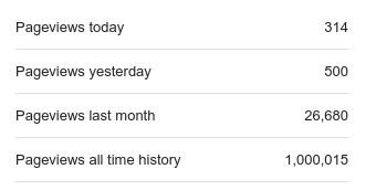
So it is a special pleasure for me to announce that, early Sunday morning (November 1, 2015), this blog reached one million page views. I am celebrating the occasion with a review of some of my favorite articles and, of course, some analysis of the page view statistics.
Here's a screenshot of my Blogger stats page to make it official:

And here are links to the 10 most read articles:
PostsEntryPageviewsAre first babies more likely to be late?Feb 7, 2011, 9 comments130446
All your Bayes are belong to us!Oct 27, 2011, 56 comments47773
My favorite Bayes's Theorem problemsOct 20, 2011, 13 comments33020
Bayesian survival analysis for "Game of Thrones"Mar 25, 2015, 5 comments32210
The Inspection Paradox is EverywhereAug 18, 2015, 23 comments30330
Bayesian statistics made simpleMar 14, 201221718
Are your data normal? Hint: no.Aug 7, 2013, 13 comments15035
Yet another reason SAT scores are non-predictiveFeb 2, 2011, 3 comments13806
Freshman hordes even more godless!Jan 29, 2012, 6 comments7904
Bayesian analysis of match rates on TinderFeb 10, 20157096
By far the most popular is my article about whether first babies are more likely to be late. It turns out they are, but only by a couple of days.
Two of the top 10 are articles written by students in my Bayesian statistics class: "Bayesian survival analysis for Game of Thrones" by Erin Pierce and Ben Kahle, and "Bayesian analysis of match rates on Tinder", by Ankur Das and Mason del Rosario. So congratulations, and thanks, to them!
Five of the top 10 are explicitly Bayesian, which is clearly the intersection of my interests and popular curiosity. But the other common theme is the application of statistical methods (of any kind) to questions people are interested in.
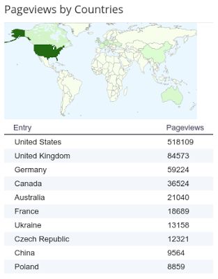
According to Blogger stats, my readers are mostly in the U.S., with most of the rest in Europe. No surprises there, with the exception of Ukraine, which is higher in the rankings than expected. Some of those views are probably bogus; anecdotally, Blogger does not do a great job of filtering robots and fake clicks (I don't have ads on my blog, so I am not sure how anyone benefits from fake clicks, but I have to conclude that some of my million are not genuine readers).
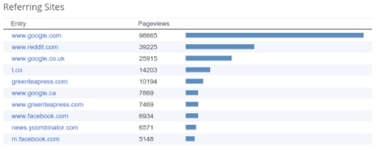
Most of my traffic comes from Google, Reddit, Twitter, and Green Tea Press, which is the home of my free books. It looks like a lot of people find me through "organic" search, as opposed to my attempts at publicity. And what are those people looking for?
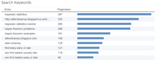
People who find my blog are looking for Bayesian statistics, apparently, and the answer to the eternal question, "Are first babies more likely to be late?"
Those are all the reports you can get from Blogger (unless you are interested in which browsers my readers use). But if I let it go at that, this blog wouldn't be called "Probably Overthinking It".
I used the Chrome extension SingleFile to grab the stats for each article in a form I can process, then used the Pandas read_html function to get it all into a table. The results, and my analysis, are in this IPython notebook.
My first post, "Proofiness and Elections", was on January 4, 2011. I've published 115 posts since then; the average time between posts is 15 days, but that includes a 180 day hiatus after "Secularization in America: Part Seven" in July 2012. I spent the fall working on Think Bayes, and got back to blogging in January 2013.
Blogger provides stats on the most popular posts; I had to do my own analysis to extract the least popular posts:

Some of these deserve their obscurity, but not all. "Will Millennials Ever Get Married?" is one of my favorite projects, and I think the video from the talk is pretty good. And "When will I win the Great Bear Run?" is one of the best statistical models I've developed, albeit applied to a problem that is mostly silly.
Measures of popularity often follow Zipf's law, and my blog is no different. As I suggest in Chapter 5 of Think Complexity, the most robust way to check for Zipf-like behavior is to plot the complementary CDF of frequency (for example, page views) on a log-log scale:
[image error]
For articles with more than 1000 page views, the CCDF is approximately straight, in compliance with Zipf's law.
The posts that elicited the most comments are:
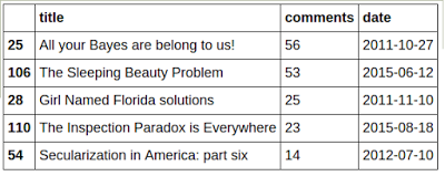
Apparently, people like their veridical paradoxes! The A few of my posts have attracted attention on the social network of Google employees, Google+:
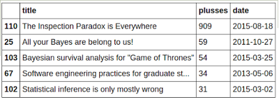
I'm glad someone appreciates The Inspection Paradox. I submitted it for publication in CHANCE magazine, but they didn't want it. Thirty thousand readers, 909 Google employees, and I think they blew it.
One thing I have learned from this blog is that I can never predict whether an article will be popular. One of the most technically challenging articles, "Bayes meets Fourier", apparently found an audience of people interested in Bayesian statistics and signal processing. At the same time, some of my favorites, like The Rock Hyrax Problem and Belly Button Biodiversity have landed flat. I've given up trying to predict what will hit.
I have posts coming up in the next few weeks that I am excited about, including an analysis of Internet use and religion using data from the European Social Survey. Watch this space.
Thanks to everyone who contributed to the first million page views. I hope you found it interesting and learned something, and I hope you'll be back for the next million!

So it is a special pleasure for me to announce that, early Sunday morning (November 1, 2015), this blog reached one million page views. I am celebrating the occasion with a review of some of my favorite articles and, of course, some analysis of the page view statistics.
Here's a screenshot of my Blogger stats page to make it official:
And here are links to the 10 most read articles:
PostsEntryPageviewsAre first babies more likely to be late?Feb 7, 2011, 9 comments130446
All your Bayes are belong to us!Oct 27, 2011, 56 comments47773
My favorite Bayes's Theorem problemsOct 20, 2011, 13 comments33020
Bayesian survival analysis for "Game of Thrones"Mar 25, 2015, 5 comments32210
The Inspection Paradox is EverywhereAug 18, 2015, 23 comments30330
Bayesian statistics made simpleMar 14, 201221718
Are your data normal? Hint: no.Aug 7, 2013, 13 comments15035
Yet another reason SAT scores are non-predictiveFeb 2, 2011, 3 comments13806
Freshman hordes even more godless!Jan 29, 2012, 6 comments7904
Bayesian analysis of match rates on TinderFeb 10, 20157096
By far the most popular is my article about whether first babies are more likely to be late. It turns out they are, but only by a couple of days.
Two of the top 10 are articles written by students in my Bayesian statistics class: "Bayesian survival analysis for Game of Thrones" by Erin Pierce and Ben Kahle, and "Bayesian analysis of match rates on Tinder", by Ankur Das and Mason del Rosario. So congratulations, and thanks, to them!
Five of the top 10 are explicitly Bayesian, which is clearly the intersection of my interests and popular curiosity. But the other common theme is the application of statistical methods (of any kind) to questions people are interested in.

According to Blogger stats, my readers are mostly in the U.S., with most of the rest in Europe. No surprises there, with the exception of Ukraine, which is higher in the rankings than expected. Some of those views are probably bogus; anecdotally, Blogger does not do a great job of filtering robots and fake clicks (I don't have ads on my blog, so I am not sure how anyone benefits from fake clicks, but I have to conclude that some of my million are not genuine readers).
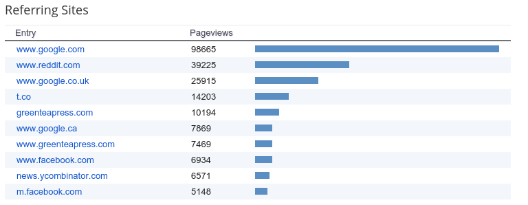
Most of my traffic comes from Google, Reddit, Twitter, and Green Tea Press, which is the home of my free books. It looks like a lot of people find me through "organic" search, as opposed to my attempts at publicity. And what are those people looking for?

People who find my blog are looking for Bayesian statistics, apparently, and the answer to the eternal question, "Are first babies more likely to be late?"
Those are all the reports you can get from Blogger (unless you are interested in which browsers my readers use). But if I let it go at that, this blog wouldn't be called "Probably Overthinking It".
I used the Chrome extension SingleFile to grab the stats for each article in a form I can process, then used the Pandas read_html function to get it all into a table. The results, and my analysis, are in this IPython notebook.
My first post, "Proofiness and Elections", was on January 4, 2011. I've published 115 posts since then; the average time between posts is 15 days, but that includes a 180 day hiatus after "Secularization in America: Part Seven" in July 2012. I spent the fall working on Think Bayes, and got back to blogging in January 2013.
Blogger provides stats on the most popular posts; I had to do my own analysis to extract the least popular posts:

Some of these deserve their obscurity, but not all. "Will Millennials Ever Get Married?" is one of my favorite projects, and I think the video from the talk is pretty good. And "When will I win the Great Bear Run?" is one of the best statistical models I've developed, albeit applied to a problem that is mostly silly.
Measures of popularity often follow Zipf's law, and my blog is no different. As I suggest in Chapter 5 of Think Complexity, the most robust way to check for Zipf-like behavior is to plot the complementary CDF of frequency (for example, page views) on a log-log scale:
[image error]
For articles with more than 1000 page views, the CCDF is approximately straight, in compliance with Zipf's law.
The posts that elicited the most comments are:

Apparently, people like their veridical paradoxes! The A few of my posts have attracted attention on the social network of Google employees, Google+:
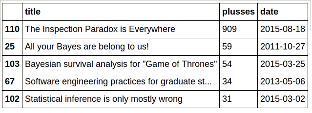
I'm glad someone appreciates The Inspection Paradox. I submitted it for publication in CHANCE magazine, but they didn't want it. Thirty thousand readers, 909 Google employees, and I think they blew it.
One thing I have learned from this blog is that I can never predict whether an article will be popular. One of the most technically challenging articles, "Bayes meets Fourier", apparently found an audience of people interested in Bayesian statistics and signal processing. At the same time, some of my favorites, like The Rock Hyrax Problem and Belly Button Biodiversity have landed flat. I've given up trying to predict what will hit.
I have posts coming up in the next few weeks that I am excited about, including an analysis of Internet use and religion using data from the European Social Survey. Watch this space.
Thanks to everyone who contributed to the first million page views. I hope you found it interesting and learned something, and I hope you'll be back for the next million!
October 26, 2015
When will I win the Great Bear Run?
Almost every year since 2008 I have participated in the Great Bear Run, a 5K road race in Needham MA. I usually finish in the top 40 or so, and in my age group I have come in 4th, 6th, 4th, 3rd, 2nd, 4th and 4th. In 2015 I didn't run because of a scheduling conflict, but based on the results I estimate that I would have come 4th again.
Having come close in 2012, I have to wonder what my chances are of winning my age group. I've developed two models to predict the results.
Binomial modelAccording to a simple binomial model (the details are in this IPython notebook), the predictive distribution for the number of people who finish ahead of me is:
[image error]
And my chances of winning my age group are about 5%.
An improved modelThe binomial model ignores an important piece of information: some of the people who have displaced me from my rightful victory have come back year after year. Here are the people who have finished ahead of me in my age group:
2008: Gardiner, McNatt, Terry
2009: McNatt, Ryan, Partridge, Turner, Demers
2010: Gardiner, Barrett, Partridge
2011: Barrett, Partridge
2012: Sagar
2013: Hammer, Wang, Hahn
2014: Partridge, Hughes, Smith
2015: Barrett, Sagar, Fernandez
Several of them are repeat interlopers. I have developed a model that takes this information into account and predicts my chances of winning. It is based on the assumption that there is a population of n runners who could displace me, each with some probability p.
In order to displace me, a runner has to
Show up,Outrun me, andBe in my age group.
For each runner, the probability of displacing me is a product of these factors:
pi=SOB
Some runners have a higher SOB factor than others; we can use previous results to estimate it.
First we have to think about an appropriate prior. Again, the details are in this IPython notebook.
Based on my experience, I conjecture that the prior distribution of S is an increasing function, with many people who run nearly every year, and fewer who run only occasionally.The prior distribution of O is biased toward high values. Of the people who have the potential to beat me, many of them will beat me every time. I am only competitive with a few of them. (For example, of the 15 people who have beat me, I have only ever beat 2).The probability that a runner is in my age group depends on the difference between his age and mine. Someone exactly my age will always be in my age group. Someone 4 years older will be in my age group only once every 5 years (the Great Bear run uses 5-year age groups). So the distribution of B is uniform.I used Beta distributions for each of the three factors, so each piis the product of three Beta-distributed variates. In general, the result is not a Beta distribution, but it turns out there is a Beta distribution that is a good approximation of the actual distribution.
[image error]
Using this distribution as a prior, we can compute the posterior distribution of p for each runner who has displaced me, and another posterior for any hypothetical runner who has not displaced me in any of 8 races. As an example, for Rich Partridge, who has displaced me in 4 of 8 years, the mean of the posterior distribution is 42%. For a runner who has only displaced me once, it is 17%.
Then, for any hypothetical number of runners, n, we can draw samples from these distributions of p and compute the conditional distribution of k, the number of runners who finish ahead of me. Here's what that looks like for a few values of n:
[image error]
If there are 18 runners, the mostly likely value of k is 3, so I would come in 4th. As the number of runners increases, my prospects look a little worse.
These represent distributions of k conditioned on n, so we can use them to compute the likelihood of the observed values of k. Then, using Bayes theorem, we can compute the posterior distribution of n, which looks like this:
[image error]
It's noisy because I used random sampling to estimate the conditional distributions of k. But that's ok because we don't really care about n; we care about the predictive distribution of k. And noise in the distribution of n has very little effect on k.
The predictive distribution of k is a weighted mixture of the conditional distributions we already computed, and it looks like this:
[image error]
Sadly, according to this model, my chance of winning my age group is less than 2% (compared to the binomial model, which predicts that my chances are more than 5%).
And one more time, the details are in this IPython notebook.
October 23, 2015
Bayes meets Fourier
Joseph Fourier never met Thomas Bayes—Fourier was born in 1768, seven years after Bayes died. But recently I have been exploring connections between the Bayes filter and the Fourier transform.
By "Bayes filter", I don't mean spam filtering using a Bayesian classifier, but rather recursive Bayesian estimation, which is used in robotics and other domains to estimate the state of a system that evolves over time, for example, the position of a moving robot. My interest in this topic was prompted by Roger Labbe's book, Kalman and Bayesian Filters in Python, which I am reading with my book club.
The Python code for this article is in this IPython notebook. If you get sick of the math, you might want to jump into the code.
The Bayes filterA Bayes filter starts with a distribution that represents probabilistic beliefs about the initial position of the robot. It proceeds by alternately executing predict and update steps:
The predict step uses a physical model of the system and its current state to predict the state in the future. For example, given the position and velocity of the robot, you could predict its location at the next time step.The update step uses a measurement and a model of measurement error to update beliefs about the state of the system. For example, if we use GPS to measure the location of the robot, the measurement would include some error, and we could characterize the distribution of errors.
The update step uses Bayes theorem, so computationally it involves multiplying the prior distribution by the likelihood distribution and then renormalizing.
The predict step involves adding random variables, like position and velocity, so computationally it involves the convolution of two distributions.
The Convolution TheoremThe Convolution Theorem suggests a symmetry between the predict and update steps, which leads to an efficient algorithm. I present the Convolution Theorem in Chapter 8 of Think DSP. For discrete signals, it says:
DFT(f ∗ g) = DFT(f) · DFT(g)
That is, if you want to compute the discrete Fourier transform (DFT) of a convolution, you can compute the DFT of the signals separately and then multiply the results. In words, convolution in the time domain corresponds to multiplication in the frequency domain. And conversely, multiplication in the time domain corresponds to convolution in the frequency domain.
In the context of Bayes filters, we are working with spatial distributions rather than temporal signals, but the convolution theorem applies: instead of the "time domain", we have the "space domain", and instead of the DFT, we have the characteristic function.
The characteristic functionThis section shows that the characteristic function and the Fourier transform are the same thing. If you already knew that, you can skip to the next section.
If you took mathematical statistics, you might have seen this definition of the characteristic function:
![\varphi_X(t) = \operatorname{E} \left [ e^{itX} \right ]](https://i.gr-assets.com/images/S/compressed.photo.goodreads.com/hostedimages/1445665200i/16689032.png)
Where X is a random variable, t is a transform variable that corresponds to frequency (temporal, spatial, or otherwise), and E is the expectation operator.
If you took signals and systems, you saw this definition of the Fourier transform:
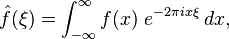
where f is a function, is its Fourier transform, and ξ is a transform variable that corresponds to a frequency.
The two definitions look different, but if you write out the expectation operator, you get

where p(x) is the probability density function of X, and P(t) is its Fourier transform. The only difference between the characteristic function and the Fourier transform is the sign of the exponent, which is just a convention choice. (The bar above P(t) indicates the complex conjugate, which is there because of the sign of the exponent.)
And that brings us to the whole point of the characteristic function: to add two random variables, you have to convolve their distributions. By the Convolution Theorem, convolution in the space domain corresponds to multiplication in the frequency domain, so you can add random variables like this:Compute the characteristic function of both distributions.Multiply the characteristic functions elementwise.Apply the inverse transform to compute the distribution of the sum.Back to BayesNow we can see the symmetry between the predict and update steps more clearly:The predict step involves convolution in the space domain, which corresponds to multiplication in the frequency domain.The update step involves multiplication in the space domain, which corresponds to convolution in the frequency domain.This observation is interesting, at least to me, and possibly useful, because it suggests an efficient algorithm based on the Fast Fourier Transform (FFT). The simple implementation of convolution takes time proportional to N², where N is the number of values in the distributions. Using the FFT, we can get that down to N log N.
Using this algorithm, a complete predict-update step looks like this:Compute the FFT of the distributions for position and velocity.Multiply them elementwise; the result is the characteristic function of the convolved distributions.Compute the inverse FFT of the result, which is the predictive distribution.Multiply the predictive distribution by the likelihood and renormalize.Steps 1 and 3 are N log N; steps 2 and 4 are linear.
I demonstrate this algorithm in this IPython notebook.
For more on the Bayesian part of the Bayes filter, you might want to read Chapter 6 of Think Bayes. For more on the Convolution Theorem, see Chapter 8 of Think DSP. And for more about adding random variables, see Chapter 6 of Think Stats.
AcknowledgementsThanks to Paul Ruvolo, the other member of my very exclusive reading club, and Wikipedia for the typeset equations I borrowed.

By "Bayes filter", I don't mean spam filtering using a Bayesian classifier, but rather recursive Bayesian estimation, which is used in robotics and other domains to estimate the state of a system that evolves over time, for example, the position of a moving robot. My interest in this topic was prompted by Roger Labbe's book, Kalman and Bayesian Filters in Python, which I am reading with my book club.
The Python code for this article is in this IPython notebook. If you get sick of the math, you might want to jump into the code.
The Bayes filterA Bayes filter starts with a distribution that represents probabilistic beliefs about the initial position of the robot. It proceeds by alternately executing predict and update steps:
The predict step uses a physical model of the system and its current state to predict the state in the future. For example, given the position and velocity of the robot, you could predict its location at the next time step.The update step uses a measurement and a model of measurement error to update beliefs about the state of the system. For example, if we use GPS to measure the location of the robot, the measurement would include some error, and we could characterize the distribution of errors.
The update step uses Bayes theorem, so computationally it involves multiplying the prior distribution by the likelihood distribution and then renormalizing.
The predict step involves adding random variables, like position and velocity, so computationally it involves the convolution of two distributions.
The Convolution TheoremThe Convolution Theorem suggests a symmetry between the predict and update steps, which leads to an efficient algorithm. I present the Convolution Theorem in Chapter 8 of Think DSP. For discrete signals, it says:
DFT(f ∗ g) = DFT(f) · DFT(g)
That is, if you want to compute the discrete Fourier transform (DFT) of a convolution, you can compute the DFT of the signals separately and then multiply the results. In words, convolution in the time domain corresponds to multiplication in the frequency domain. And conversely, multiplication in the time domain corresponds to convolution in the frequency domain.
In the context of Bayes filters, we are working with spatial distributions rather than temporal signals, but the convolution theorem applies: instead of the "time domain", we have the "space domain", and instead of the DFT, we have the characteristic function.
The characteristic functionThis section shows that the characteristic function and the Fourier transform are the same thing. If you already knew that, you can skip to the next section.
If you took mathematical statistics, you might have seen this definition of the characteristic function:
Where X is a random variable, t is a transform variable that corresponds to frequency (temporal, spatial, or otherwise), and E is the expectation operator.
If you took signals and systems, you saw this definition of the Fourier transform:
where f is a function,
is its Fourier transform, and ξ is a transform variable that corresponds to a frequency.The two definitions look different, but if you write out the expectation operator, you get
where p(x) is the probability density function of X, and P(t) is its Fourier transform. The only difference between the characteristic function and the Fourier transform is the sign of the exponent, which is just a convention choice. (The bar above P(t) indicates the complex conjugate, which is there because of the sign of the exponent.)
And that brings us to the whole point of the characteristic function: to add two random variables, you have to convolve their distributions. By the Convolution Theorem, convolution in the space domain corresponds to multiplication in the frequency domain, so you can add random variables like this:Compute the characteristic function of both distributions.Multiply the characteristic functions elementwise.Apply the inverse transform to compute the distribution of the sum.Back to BayesNow we can see the symmetry between the predict and update steps more clearly:The predict step involves convolution in the space domain, which corresponds to multiplication in the frequency domain.The update step involves multiplication in the space domain, which corresponds to convolution in the frequency domain.This observation is interesting, at least to me, and possibly useful, because it suggests an efficient algorithm based on the Fast Fourier Transform (FFT). The simple implementation of convolution takes time proportional to N², where N is the number of values in the distributions. Using the FFT, we can get that down to N log N.
Using this algorithm, a complete predict-update step looks like this:Compute the FFT of the distributions for position and velocity.Multiply them elementwise; the result is the characteristic function of the convolved distributions.Compute the inverse FFT of the result, which is the predictive distribution.Multiply the predictive distribution by the likelihood and renormalize.Steps 1 and 3 are N log N; steps 2 and 4 are linear.
I demonstrate this algorithm in this IPython notebook.
For more on the Bayesian part of the Bayes filter, you might want to read Chapter 6 of Think Bayes. For more on the Convolution Theorem, see Chapter 8 of Think DSP. And for more about adding random variables, see Chapter 6 of Think Stats.
AcknowledgementsThanks to Paul Ruvolo, the other member of my very exclusive reading club, and Wikipedia for the typeset equations I borrowed.
September 23, 2015
First babies are more likely to be late
If you are pregnant with your first child, you might have heard that first babies are more likely to be late. This turns out to be true, although the difference is small.
Averaged across all live births, the mean gestation for first babies is 38.6 weeks, compared to 38.5 weeks for other babies. This difference is about 16 hours.
Those means include pre-term babies, which affect the averages in a way that understates the difference. For full-term babies, the differences are a little bigger.
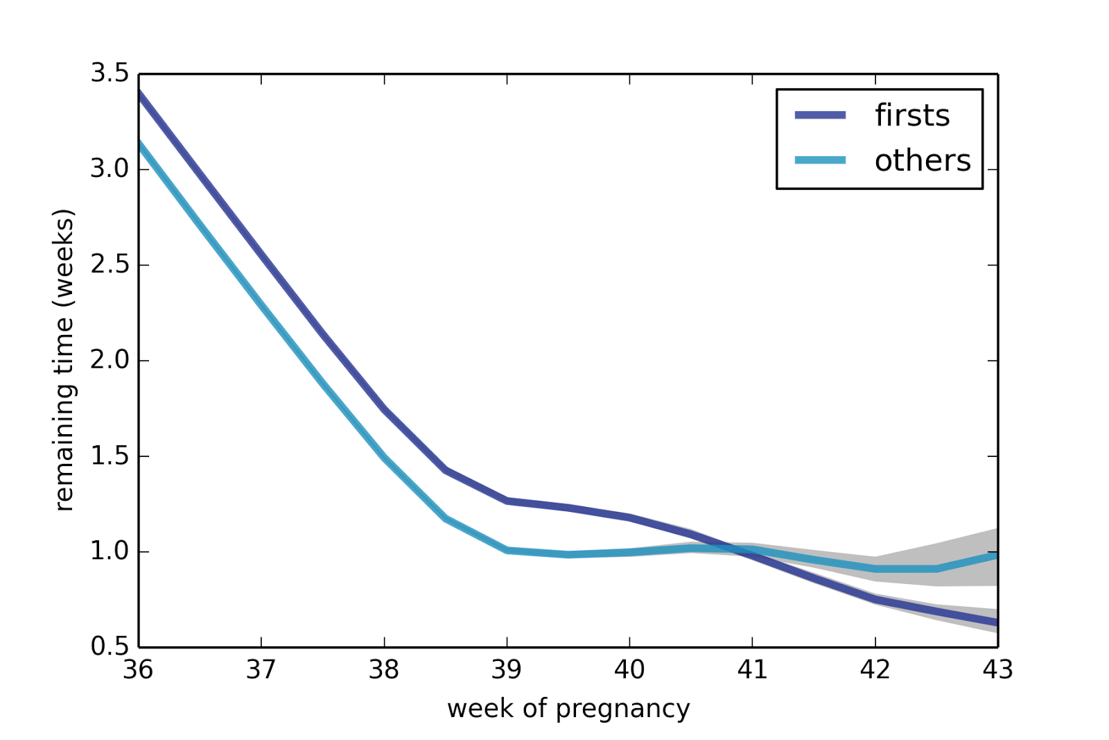
For example, if you are at the beginning of week 36, the average time until delivery is 3.4 weeks for first babies and 3.1 weeks for others, a difference of 1.8 days. The gap is about the same for weeks 37 through 40. After that, there is no consistent difference between first babies and others.
The following figure shows average remaining duration in weeks, for first babies and others, computed for weeks 36 through 43.
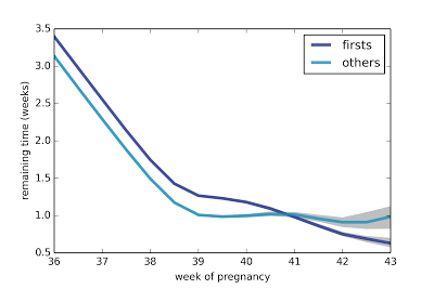
The gap between first babies and others is consistent until Week 41. As an aside, this figure also shows a surprising pattern: after Week 38, the expected remaining duration levels off at about one week. For more than a month, the finish line is always a week away!
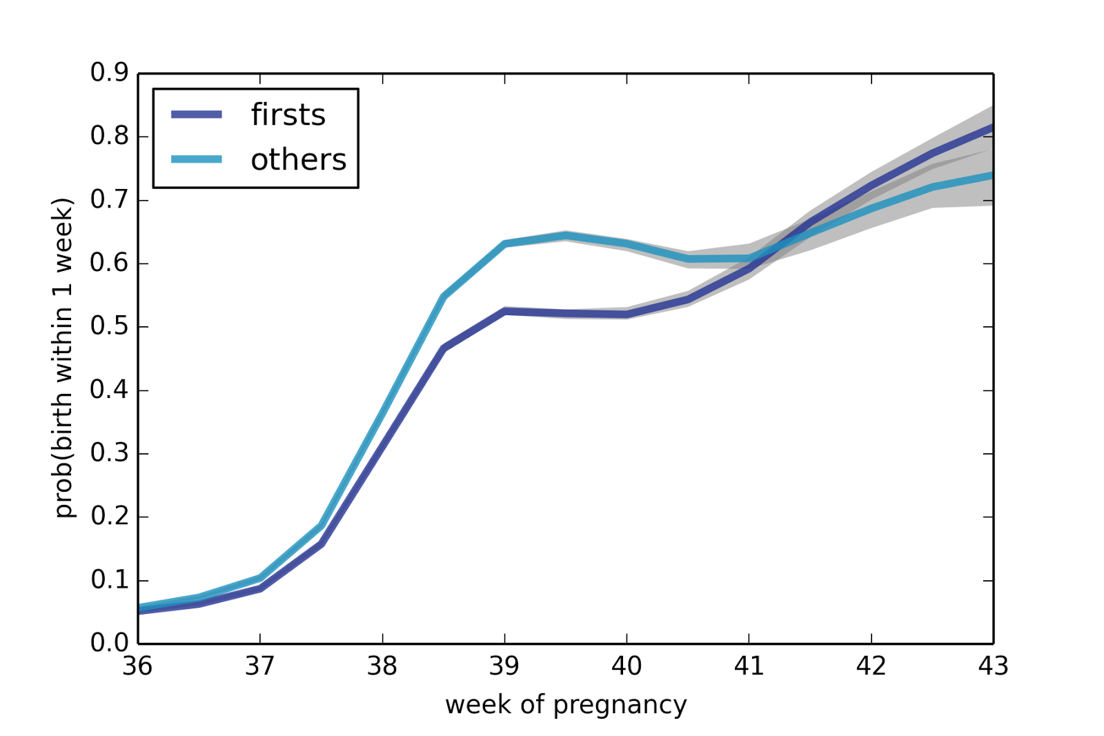
Looking at the probability of delivering in the next week, we see a similar pattern: from Week 38 on, the probability is almost the same, with some increase after Week 41.
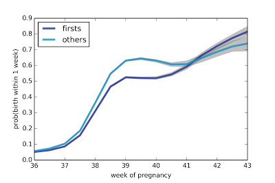
The difference between first babies and others is highest in Weeks 39 and 40; for example, in Week 39, the chance of delivering in the next week is 52% for first babies, compared to 64% for others. By Week 41, this gap has closed.
In summary, among full-term pregnancies, first babies arrive a little later than others, by about two days. After Week 38, the expected remaining duration is about one week.
Methods
The code I used to generate these results is in this IPython Notebook. I used data from the National Survey of Family Growth (NSFG). During the last three survey cycles, they interviewed more than 25,000 women and collected data about more than 48,000 pregnancies. Of those, I selected the 30,110 pregnancies whose outcome was a live birth.
Of those, there were 13,864 first babies and 16,246 others. The mean gestation period for first babies is 38.61, with SE 0.024; for others it is 38.52 with SE 0.019. The difference is statistically significant with p < 0.001.
However, those means could be misleading for two reasons: they include pre-term babies, which bring down the averages for both groups. Also, they do not take into account the stratified survey design.
To address the second point, I use weighted resampling, running each analysis 101 times and selecting the 10th, 50th, and 90th percentile of the results. The lines in the figure above show median values (50th percentile). The gray areas show an 80% confidence interval (between the 10th and 90th percentiles).
Background
I use this question—whether first babies are more likely to be late—as a case study in my book, Think Stats . There, I used data from only one cycle of the NSFG. I report a small difference between first babies and others, but it is not statistically significant.
I also wrote about this question in a previous blog article, "Are first babies more likely to be late?", which has been viewed more than 100,000 times, more than any other article on this blog.
I am reviewing the question now for two reasons:
1) I worked on another project that required me to load data from other cycles of the NSFG. Having done that work, I saw an opportunity to run my analysis again with more data.
2) Since my previous articles were intended partly for statistics education, I kept the analysis simple. In particular, I ignored the stratified design of the survey, which made the results suspect. Fortunately, it turns out that the effect is small; the new results are consistent with what I saw before.
Since I've been writing about this topic and using it as a teaching example for more than 5 years, I hope the question is settled now.

Averaged across all live births, the mean gestation for first babies is 38.6 weeks, compared to 38.5 weeks for other babies. This difference is about 16 hours.
Those means include pre-term babies, which affect the averages in a way that understates the difference. For full-term babies, the differences are a little bigger.
For example, if you are at the beginning of week 36, the average time until delivery is 3.4 weeks for first babies and 3.1 weeks for others, a difference of 1.8 days. The gap is about the same for weeks 37 through 40. After that, there is no consistent difference between first babies and others.
The following figure shows average remaining duration in weeks, for first babies and others, computed for weeks 36 through 43.
The gap between first babies and others is consistent until Week 41. As an aside, this figure also shows a surprising pattern: after Week 38, the expected remaining duration levels off at about one week. For more than a month, the finish line is always a week away!
Looking at the probability of delivering in the next week, we see a similar pattern: from Week 38 on, the probability is almost the same, with some increase after Week 41.
The difference between first babies and others is highest in Weeks 39 and 40; for example, in Week 39, the chance of delivering in the next week is 52% for first babies, compared to 64% for others. By Week 41, this gap has closed.
In summary, among full-term pregnancies, first babies arrive a little later than others, by about two days. After Week 38, the expected remaining duration is about one week.
Methods
The code I used to generate these results is in this IPython Notebook. I used data from the National Survey of Family Growth (NSFG). During the last three survey cycles, they interviewed more than 25,000 women and collected data about more than 48,000 pregnancies. Of those, I selected the 30,110 pregnancies whose outcome was a live birth.
Of those, there were 13,864 first babies and 16,246 others. The mean gestation period for first babies is 38.61, with SE 0.024; for others it is 38.52 with SE 0.019. The difference is statistically significant with p < 0.001.
However, those means could be misleading for two reasons: they include pre-term babies, which bring down the averages for both groups. Also, they do not take into account the stratified survey design.
To address the second point, I use weighted resampling, running each analysis 101 times and selecting the 10th, 50th, and 90th percentile of the results. The lines in the figure above show median values (50th percentile). The gray areas show an 80% confidence interval (between the 10th and 90th percentiles).
Background
I use this question—whether first babies are more likely to be late—as a case study in my book, Think Stats . There, I used data from only one cycle of the NSFG. I report a small difference between first babies and others, but it is not statistically significant.
I also wrote about this question in a previous blog article, "Are first babies more likely to be late?", which has been viewed more than 100,000 times, more than any other article on this blog.
I am reviewing the question now for two reasons:
1) I worked on another project that required me to load data from other cycles of the NSFG. Having done that work, I saw an opportunity to run my analysis again with more data.
2) Since my previous articles were intended partly for statistics education, I kept the analysis simple. In particular, I ignored the stratified design of the survey, which made the results suspect. Fortunately, it turns out that the effect is small; the new results are consistent with what I saw before.
Since I've been writing about this topic and using it as a teaching example for more than 5 years, I hope the question is settled now.
September 1, 2015
Bayesian analysis of gluten sensitivity
Last week a new study showed that many subjects diagnosed with non-celiac gluten sensitivity (NCGS) were not able to distinguish gluten flour from non-gluten flour in a blind challenge.
In this article, I review the the study and use a simple Bayesian model to show that the results support the hypothesis that none of the subjects are sensitive to gluten. But there are complications in the design of the study that might invalidate the model.
Here is a description of the study:
This conclusion seems odd to me, because if none of the patients were sensitive to gluten, we would expect some of them to identify the gluten flour by chance. So the results are consistent with the hypothesis that none of the subjects are actually gluten sensitive.
We can use a Bayesian approach to interpret the results more precisely. But first, as always, we have to make some modeling decisions.
First, of the 35 subjects, 12 identified the gluten flour based on resumption of symptoms while they were eating it. Another 17 subjects wrongly identified the gluten-free flour based on their symptoms, and 6 subjects were unable to distinguish. So each subject gave one of three responses. To keep things simple I follow the authors of the study and lump together the second two groups; that is, I consider two groups: those who identified the gluten flour and those who did not.
Second, I assume (1) people who are actually gluten sensitive have a 95% chance of correctly identifying gluten flour under the challenge conditions, and (2) subjects who are not gluten sensitive have only a 40% chance of identifying the gluten flour by chance (and a 60% chance of either choosing the other flour or failing to distinguish).
Under this model, we can estimate the actual number of subjects who are gluten sensitive, gs. I chose a uniform prior for gs, from 0 to 35. To perform the Bayesian analysis, we have to compute the likelihood of the data under each hypothetical value of gs. Here is the likelihood function in Python
def Likelihood(self, data, hypo):
gs = hypo
yes, no = data
n = yes + no
ngs = n - gs
pmf1 = thinkbayes2.MakeBinomialPmf(gs, 0.95)
pmf2 = thinkbayes2.MakeBinomialPmf(ngs, 0.4)
pmf = pmf1 + pmf2
return pmf[yes]
The function works by computing the PMF of the number of gluten identifications conditioned on gs, and then selecting the actual number of identifications, yes, from the PMF. The details of the computation are in this IPython notebook.
And here is the posterior distribution:

The most likely value of gs is 0, so it is quite possible that none of the respondents are gluten sensitive. The 95% credible interval for gs is (0, 8), so a reasonable upper bound on the number of gluten-sensitive respondents is 8 out of 35, or 23%.
We can also use this analysis to compare two hypotheses:
A) Some of the respondents are gluten sensitive (equally likely from 0 to 35).
B) None of the respondents are gluten sensitive.
The Bayes factor in support of B turns out to be about 8.4, which is moderately strong. If you believed, before reading this study, that the probability of B was 50%, you should now believe it is about 90%.
However, there are complications in the design of the study that might invalidate this simple model. In particular, the gluten free flour in the study contained corn starch, which some people may be sensitive to. And several subjects reported symptoms under both challenge conditions; that is, when eating both gluten flour and gluten-free flour. So it is possible that misidentification of the gluten flour, as well as failure to distinguish, indicates sensitivity to both gluten and corn starch.
But if we limit ourselves to the question of whether people diagnosed with non-celiac gluten sensitivity are specifically sensitive to gluten, this study suggests that they are not.
Thank yous: I heard about this study in this blog post. And I want to thank the authors of the study and their publisher for making the entire paper available on the web, which made my analysis possible.

In this article, I review the the study and use a simple Bayesian model to show that the results support the hypothesis that none of the subjects are sensitive to gluten. But there are complications in the design of the study that might invalidate the model.
Here is a description of the study:
"We studied 35 non-CD subjects (31 females) that were on a gluten-free diet (GFD), in a double-blind challenge study. Participants were randomised to receive either gluten-containing flour or gluten-free flour for 10 days, followed by a 2-week washout period and were then crossed over. The main outcome measure was their ability to identify which flour contained gluten.Since 12 out of 35 participants were able to identify the gluten flour, the authors conclude "Double-blind gluten challenge induces symptom recurrence in just one-third of patients fulfilling the clinical diagnostic criteria for non-coeliac gluten sensitivity."
"The gluten-containing flour was correctly identified by 12 participants (34%)..."
This conclusion seems odd to me, because if none of the patients were sensitive to gluten, we would expect some of them to identify the gluten flour by chance. So the results are consistent with the hypothesis that none of the subjects are actually gluten sensitive.
We can use a Bayesian approach to interpret the results more precisely. But first, as always, we have to make some modeling decisions.
First, of the 35 subjects, 12 identified the gluten flour based on resumption of symptoms while they were eating it. Another 17 subjects wrongly identified the gluten-free flour based on their symptoms, and 6 subjects were unable to distinguish. So each subject gave one of three responses. To keep things simple I follow the authors of the study and lump together the second two groups; that is, I consider two groups: those who identified the gluten flour and those who did not.
Second, I assume (1) people who are actually gluten sensitive have a 95% chance of correctly identifying gluten flour under the challenge conditions, and (2) subjects who are not gluten sensitive have only a 40% chance of identifying the gluten flour by chance (and a 60% chance of either choosing the other flour or failing to distinguish).
Under this model, we can estimate the actual number of subjects who are gluten sensitive, gs. I chose a uniform prior for gs, from 0 to 35. To perform the Bayesian analysis, we have to compute the likelihood of the data under each hypothetical value of gs. Here is the likelihood function in Python
def Likelihood(self, data, hypo):
gs = hypo
yes, no = data
n = yes + no
ngs = n - gs
pmf1 = thinkbayes2.MakeBinomialPmf(gs, 0.95)
pmf2 = thinkbayes2.MakeBinomialPmf(ngs, 0.4)
pmf = pmf1 + pmf2
return pmf[yes]
The function works by computing the PMF of the number of gluten identifications conditioned on gs, and then selecting the actual number of identifications, yes, from the PMF. The details of the computation are in this IPython notebook.
And here is the posterior distribution:
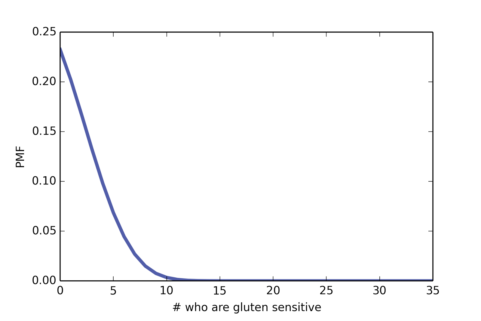
The most likely value of gs is 0, so it is quite possible that none of the respondents are gluten sensitive. The 95% credible interval for gs is (0, 8), so a reasonable upper bound on the number of gluten-sensitive respondents is 8 out of 35, or 23%.
We can also use this analysis to compare two hypotheses:
A) Some of the respondents are gluten sensitive (equally likely from 0 to 35).
B) None of the respondents are gluten sensitive.
The Bayes factor in support of B turns out to be about 8.4, which is moderately strong. If you believed, before reading this study, that the probability of B was 50%, you should now believe it is about 90%.
However, there are complications in the design of the study that might invalidate this simple model. In particular, the gluten free flour in the study contained corn starch, which some people may be sensitive to. And several subjects reported symptoms under both challenge conditions; that is, when eating both gluten flour and gluten-free flour. So it is possible that misidentification of the gluten flour, as well as failure to distinguish, indicates sensitivity to both gluten and corn starch.
But if we limit ourselves to the question of whether people diagnosed with non-celiac gluten sensitivity are specifically sensitive to gluten, this study suggests that they are not.
Thank yous: I heard about this study in this blog post. And I want to thank the authors of the study and their publisher for making the entire paper available on the web, which made my analysis possible.
August 27, 2015
Bayes theorem in real life
I had a chance to practice Bayesian inference in real life today: at 1pm my wife called to tell me that the carbon monoxide (CO) alarm at the house was going off. Immediately two hypotheses came to mind: (1) there is a dangerous amount of CO in my house, (2) it's a false alarm.
It's summer and all the windows are open in the house. The furnace is not running and we don't have a gas stove. And the detector is about 10 years old. This background information makes a false alarm more plausible, so I started with a low prior for (1). Since my wife was on her way out anyway, I suggested she disconnect the detector, turn on a fan, and leave.
After we hung up, I searched for information on CO detectors and false alarms. Apparently, the rate of false alarms is low, at least in once sense: CO detectors are very specific, that is, unlikely to go off because of anything other than CO. Of course the other possibility is that the detector is broken. On balance, this information made me less confident of a false alarm.
I tried to think of other possibilities:
A major street nearby is being paved. Does fresh pavement off-gas anything that would set off a CO detector?At a construction site down the street, they just poured a concrete foundation, and my neighbor is having some masonry done. Does fresh concrete off-gas CO? I vaguely remember that it sequesters oxygen, which turned out to be a problem for one of the Biosphere projects.What about a smoldering fire inside a wall? Could it produce enough CO to set off the detector, but not enough smoke to set off the smoke alarms?The first two seemed unlikely, but the third seemed plausible. In fact, it seemed plausible enough that I decided to go home and check it out. When I got there, the windows were open and fans were running, so I figured the air had exchanged at least once, and the detector had a chance to reset.
I put on over-the-head 30dB earmuffs and plugged the detector back in. It went off immediately. I plugged it into an outlet in another room, and it went off immediately. At this point it seemed unlikely that every room in my wide-open, highly ventilated house was full of CO.
I still couldn't rule out a smoldering fire, but it sure seemed unlikely. Nevertheless, I called the fire department, using their non-emergency number to preserve some dignity, and told them the story. They sent a truck, walked through the house with a gas detector, and reported no CO anywhere.
One of the fireman told me that CO detectors are good for about 7 years, so it's time for a new one. And while I'm at it, he suggested, I should get one more for the first floor (currently I have one in the basement and one on the second floor). And that's what I did.
So what have we learned?
1) Make sure you have a CO detector on each floor of your house. CO poisoning is no joke. Want proof? Run this search query any time. Chances are you'll find several serious accidents within the last week or so.
2) Replace detectors after 5-7 years. Apparently newer ones have an end-of-life alert, so you don't have to keep track. If you have an older one, figure out the replacement day and put it on your calendar.
3) Think like a Bayesian. As you get more information, update your probabilities, and change your decisions accordingly. My initial estimate for the probability of false alarm was so high, I decided not to check it out. As I thought of more possible explanations, the probability of a real problem crept higher. It was still very low, but high enough that I decided to go home.
4) On the other hand, a strictly Bayesian framework doesn't always fit real-world thinking. In this case, my decision flipped when I thought of a new hypothesis (a smoldering fire). Should I consider that a new piece of information and update my prior? Or is it a new piece of background information that caused me to go back, revise my prior, and start over? In practice, it makes no difference. But from a Bayesian point of view, it's not quite as neat as it might be.
August 18, 2015
The Inspection Paradox is Everywhere
The following is a draft of an article I have submitted for publication in CHANCE Magazine, a publication of the American Statistical Association. With their encouragement, I am publishing it here to solicit comments from readers (and possibly corrections).
The Inspection Paradox is Everywhere
The inspection paradox is a common source of confusion, an occasional source of error, and an opportunity for clever experimental design. Most people are unaware of it, but like the cue marks that appear in movies to signal reel changes, once you notice it, you can’t stop seeing it.
A common example is the apparent paradox of class sizes. Suppose you ask college students how big their classes are and average the responses. The result might be 56. But if you ask the school for the average class size, they might say 31. It sounds like someone is lying, but they could both be right.
The problem is that when you survey students, you oversample large classes. If are 10 students in a class, you have 10 chances to sample that class. If there are 100 students, you have 100 chances. In general, if the class size is x, it will be overrepresented in the sample by a factor of x.
That’s not necessarily a mistake. If you want to quantify student experience, the average across students might be a more meaningful statistic than the average across classes. But you have to be clear about what you are measuring and how you report it.
By the way, I didn’t make up the numbers in this example. They come from class sizes reported by Purdue University for undergraduate classes in the 2013-14 academic year. https://www.purdue.edu/datadigest/2013-14/InstrStuLIfe/DistUGClasses.html
From the data in their report, I estimate the actual distribution of class sizes; then I compute the “biased” distribution you would get by sampling students. The CDFs of these distributions are in Figure 1.
Going the other way, if you are given the biased distribution, you can invert the process to estimate the actual distribution. You could use this strategy if the actual distribution is not available, or if it is easier to run the biased sampling process.
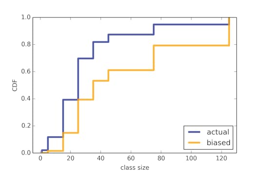 Figure 1: Undergraduate class sizes at Purdue University, 2013-14 academic year: actual distribution and biased view as seen by students.
The same effect applies to passenger planes. Airlines complain that they are losing money because too many flights are nearly empty. At the same time passengers complain that flying is miserable because planes are too full. They could both be right. When a flight is nearly empty, only a few passengers enjoy the extra space. But when a flight is full, many passengers feel the crunch.
Once you notice the inspection paradox, you see it everywhere. Does it seem like you can never get a taxi when you need one? Part of the problem is that when there is a surplus of taxis, only a few customers enjoy it. When there is a shortage, many people feel the pain.
Another example happens when you are waiting for public transportation. Busses and trains are supposed to arrive at constant intervals, but in practice some intervals are longer than others. With your luck, you might think you are more likely to arrive during a long interval. It turns out you are right: a random arrival is more likely to fall in a long interval because, well, it’s longer.
To quantify this effect, I collected data from the Red Line in Boston. Using their real-time data service, I recorded the arrival times for 70 trains between 4pm and 5pm over several days.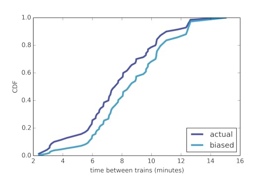 Figure 2: Distribution of time between trains on the Red Line in Boston, between 4pm and 5pm.
The shortest gap between trains was less than 3 minutes; the longest was more than 15. Figure 2 shows the actual distribution of time between trains, and the biased distribution that would be observed by passengers. The average time between trains is 7.8 minutes, so we might expect the average wait time to be 3.8 minutes. But the average of the biased distribution is 8.8 minutes, and the average wait time for passengers is 4.4 minutes, about 15% longer.
In this case the difference between the two distributions is not very big because the variance of the actual distribution is moderate. When the actual distribution is long-tailed, the effect of the inspection paradox can be much bigger.
An example of a long-tailed distribution comes up in the context of social networks. In 1991, Scott Feld presented the “friendship paradox”: the observation that most people have fewer friends than their friends have. He studied real-life friends, but the same effect appears in online networks: if you choose a random Facebook user, and then choose one of their friends at random, the chance is about 80% that the friend has more friends.
The friendship paradox is a form of the inspection paradox. When you choose a random user, every user is equally likely. But when you choose one of their friends, you are more likely to choose someone with a lot of friends. Specifically, someone with x friends is overrepresented by a factor of x.
To demonstrate the effect, I use data from the Stanford Large Network Dataset Collection (http://snap.stanford.edu/data), which includes a sample of about 4000 Facebook users. We can compute the number of friends each user has and plot the distribution, shown in Figure 3. The distribution is skewed: most users have only a few friends, but some have hundreds.
We can also compute the biased distribution we would get by choosing choosing random friends, also shown in Figure 3. The difference is huge. In this dataset, the average user has 42 friends; the average friend has more than twice as many, 91.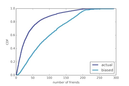 Figure 3: Number of online friends for Facebook users: actual distribution and biased distribution seen by sampling friends.
Some examples of the inspection paradox are more subtle. One of them occurred to me when I ran a 209-mile relay race in New Hampshire. I ran the sixth leg for my team, so when I started running, I jumped into the middle of the race. After a few miles I noticed something unusual: when I overtook slower runners, they were usually much slower; and when faster runners passed me, they were usually much faster.
At first I thought the distribution of runners was bimodal, with many slow runners, many fast runners, and few runners like me in the middle. Then I realized that I was fooled by the inspection paradox.
In many long relay races, teams start at different times, and most teams include a mix of faster and slower runners. As a result, runners at different speeds end up spread over the course; if you stand at random spot and watch runners go by, you see a nearly representative sample of speeds. But if you jump into the race in the middle, the sample you see depends on your speed.
Whatever speed you run, you are more likely to pass very slow runners, more likely to be overtaken by fast runners, and unlikely to see anyone running at the same speed as you. The chance of seeing another runner is proportional to the difference between your speed and theirs.
We can simulate this effect using data from a conventional road race. Figure 4 shows the actual distribution of speeds from the James Joyce Ramble, a 10K race in Massachusetts. It also shows biased distributions that would be seen by runners at 6.5 and 7.5 mph. The observed distributions are bimodal, with fast and slow runners oversampled and fewer runners in the middle.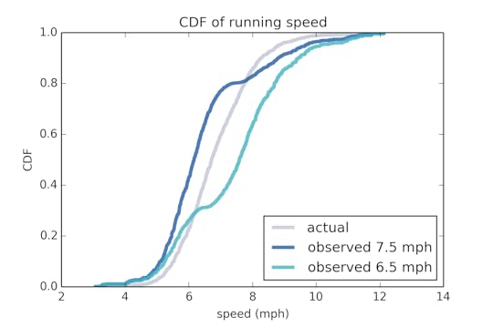 Figure 4: Distribution of speed for runners in a 10K, and biased distributions as seen by runners at different speeds.
A final example of the inspection paradox occurred to me when I was reading Orange is the New Black, a memoir by Piper Kerman, who spent 13 months in a federal prison. At several points Kerman expresses surprise at the length of the sentences her fellow prisoners are serving. She is right to be surprised, but it turns out that she is the victim of not just an inhumane prison system, but also the inspection paradox.
If you arrive at a prison at a random time and choose a random prisoner, you are more likely to choose a prisoner with a long sentence. Once again, a prisoner with sentence x is oversampled by a factor of x.
Using data from the U.S. Sentencing Commission, I made a rough estimate of the distribution of sentences for federal prisoners, shown in Figure 5. I also computed the biased distribution as observed by a random arrival.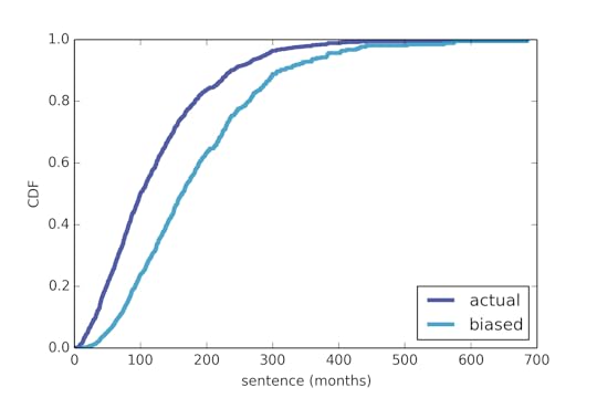 Figure 5: Approximate distribution of federal prison sentences, and a biased distribution as seen by a random arrival.
As expected, the biased distribution is shifted to the right. In the actual distibution the mean is 121 months; in the biased distribution it is 183 months.
So what happens if you observe a prison over an interval like 13 months? It turns out that if your sentence is y months, the chance of overlapping with a prisoner whose sentence is x months is proportional to x + y.
Figure 6 shows biased distributions as seen by hypothetical prisoners serving sentences of 13, 120, and 600 months.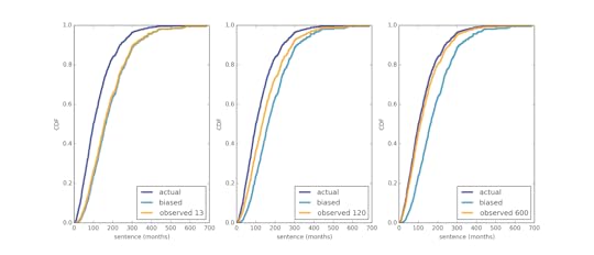 Figure 6: Biased distributions as seen by prisoners with different sentences.
Over an interval of 13 months, the observed sample is not much better than the biased sample seen by a random arrival. After 120 months, the magnitude of the bias is about halved. Only after a very long sentence, 600 months, do we get a more representative sample, and even then it is not entirely unbiased.
These examples show that the inspection paradox appears in many domains, sometimes in subtle ways. If you are not aware of it, it can cause statistical errors and lead to invalid inferences. But in many cases it can be avoided, or even used deliberately as part of an experimental design.
Further readingI discuss the class size example in my book, Think Stats, 2nd Edition, O’Reilly Media, 2014, and the Red Line example in Think Bayes, O’Reilly Media, 2013. I wrote about relay races, social networks, and Orange Is the New Black in my blog, “Probably Overthinking It”. http://allendowney.blogspot.com/
John Allen Paulos presents the friendship paradox in Scientific American, “Why You're Probably Less Popular Than Your Friends”, 18 January 2011. http://www.scientificamerican.com/article/why-youre-probably-less-popular/The original paper on the topic might be Scott Feld, “Why Your Friends Have More Friends Than You Do”, American Journal of Sociology, Vol. 96, No. 6 (May, 1991), pp. 1464-1477. http://www.jstor.org/stable/2781907
Amir Aczel discusses some of these examples, and a few different ones, in a Discover Magazine blog article, “On the Persistence of Bad Luck (and Good)”, 4 September 4, 2013.http://blogs.discovermagazine.com/crux/2013/09/04/on-the-persistence-of-bad-luck-and-good
The code I used to generate these examples is in these Jupyter notebooks:https://github.com/AllenDowney/ProbablyOverthinkingIt/blob/master/inspection.ipynbhttps://github.com/AllenDowney/ProbablyOverthinkingIt/blob/master/redline.ipynbhttps://github.com/AllenDowney/ProbablyOverthinkingIt/blob/master/social.ipynbhttps://github.com/AllenDowney/ProbablyOverthinkingIt/blob/master/relay.ipynbhttps://github.com/AllenDowney/ProbablyOverthinkingIt/blob/master/orange.ipynb
Bio
Allen Downey is a Professor of Computer Science at Olin College of Engineering in Massachusetts. He is the author of several books, including Think Python, Think Stats, and Think Bayes. He is a runner with a maximum 10K speed of 8.7 mph.

The Inspection Paradox is Everywhere
The inspection paradox is a common source of confusion, an occasional source of error, and an opportunity for clever experimental design. Most people are unaware of it, but like the cue marks that appear in movies to signal reel changes, once you notice it, you can’t stop seeing it.
A common example is the apparent paradox of class sizes. Suppose you ask college students how big their classes are and average the responses. The result might be 56. But if you ask the school for the average class size, they might say 31. It sounds like someone is lying, but they could both be right.
The problem is that when you survey students, you oversample large classes. If are 10 students in a class, you have 10 chances to sample that class. If there are 100 students, you have 100 chances. In general, if the class size is x, it will be overrepresented in the sample by a factor of x.
That’s not necessarily a mistake. If you want to quantify student experience, the average across students might be a more meaningful statistic than the average across classes. But you have to be clear about what you are measuring and how you report it.
By the way, I didn’t make up the numbers in this example. They come from class sizes reported by Purdue University for undergraduate classes in the 2013-14 academic year. https://www.purdue.edu/datadigest/2013-14/InstrStuLIfe/DistUGClasses.html
From the data in their report, I estimate the actual distribution of class sizes; then I compute the “biased” distribution you would get by sampling students. The CDFs of these distributions are in Figure 1.
Going the other way, if you are given the biased distribution, you can invert the process to estimate the actual distribution. You could use this strategy if the actual distribution is not available, or if it is easier to run the biased sampling process.
Figure 1: Undergraduate class sizes at Purdue University, 2013-14 academic year: actual distribution and biased view as seen by students.
The same effect applies to passenger planes. Airlines complain that they are losing money because too many flights are nearly empty. At the same time passengers complain that flying is miserable because planes are too full. They could both be right. When a flight is nearly empty, only a few passengers enjoy the extra space. But when a flight is full, many passengers feel the crunch.
Once you notice the inspection paradox, you see it everywhere. Does it seem like you can never get a taxi when you need one? Part of the problem is that when there is a surplus of taxis, only a few customers enjoy it. When there is a shortage, many people feel the pain.
Another example happens when you are waiting for public transportation. Busses and trains are supposed to arrive at constant intervals, but in practice some intervals are longer than others. With your luck, you might think you are more likely to arrive during a long interval. It turns out you are right: a random arrival is more likely to fall in a long interval because, well, it’s longer.
To quantify this effect, I collected data from the Red Line in Boston. Using their real-time data service, I recorded the arrival times for 70 trains between 4pm and 5pm over several days.
Figure 2: Distribution of time between trains on the Red Line in Boston, between 4pm and 5pm.
The shortest gap between trains was less than 3 minutes; the longest was more than 15. Figure 2 shows the actual distribution of time between trains, and the biased distribution that would be observed by passengers. The average time between trains is 7.8 minutes, so we might expect the average wait time to be 3.8 minutes. But the average of the biased distribution is 8.8 minutes, and the average wait time for passengers is 4.4 minutes, about 15% longer.
In this case the difference between the two distributions is not very big because the variance of the actual distribution is moderate. When the actual distribution is long-tailed, the effect of the inspection paradox can be much bigger.
An example of a long-tailed distribution comes up in the context of social networks. In 1991, Scott Feld presented the “friendship paradox”: the observation that most people have fewer friends than their friends have. He studied real-life friends, but the same effect appears in online networks: if you choose a random Facebook user, and then choose one of their friends at random, the chance is about 80% that the friend has more friends.
The friendship paradox is a form of the inspection paradox. When you choose a random user, every user is equally likely. But when you choose one of their friends, you are more likely to choose someone with a lot of friends. Specifically, someone with x friends is overrepresented by a factor of x.
To demonstrate the effect, I use data from the Stanford Large Network Dataset Collection (http://snap.stanford.edu/data), which includes a sample of about 4000 Facebook users. We can compute the number of friends each user has and plot the distribution, shown in Figure 3. The distribution is skewed: most users have only a few friends, but some have hundreds.
We can also compute the biased distribution we would get by choosing choosing random friends, also shown in Figure 3. The difference is huge. In this dataset, the average user has 42 friends; the average friend has more than twice as many, 91.
Figure 3: Number of online friends for Facebook users: actual distribution and biased distribution seen by sampling friends.
Some examples of the inspection paradox are more subtle. One of them occurred to me when I ran a 209-mile relay race in New Hampshire. I ran the sixth leg for my team, so when I started running, I jumped into the middle of the race. After a few miles I noticed something unusual: when I overtook slower runners, they were usually much slower; and when faster runners passed me, they were usually much faster.
At first I thought the distribution of runners was bimodal, with many slow runners, many fast runners, and few runners like me in the middle. Then I realized that I was fooled by the inspection paradox.
In many long relay races, teams start at different times, and most teams include a mix of faster and slower runners. As a result, runners at different speeds end up spread over the course; if you stand at random spot and watch runners go by, you see a nearly representative sample of speeds. But if you jump into the race in the middle, the sample you see depends on your speed.
Whatever speed you run, you are more likely to pass very slow runners, more likely to be overtaken by fast runners, and unlikely to see anyone running at the same speed as you. The chance of seeing another runner is proportional to the difference between your speed and theirs.
We can simulate this effect using data from a conventional road race. Figure 4 shows the actual distribution of speeds from the James Joyce Ramble, a 10K race in Massachusetts. It also shows biased distributions that would be seen by runners at 6.5 and 7.5 mph. The observed distributions are bimodal, with fast and slow runners oversampled and fewer runners in the middle.
Figure 4: Distribution of speed for runners in a 10K, and biased distributions as seen by runners at different speeds.
A final example of the inspection paradox occurred to me when I was reading Orange is the New Black, a memoir by Piper Kerman, who spent 13 months in a federal prison. At several points Kerman expresses surprise at the length of the sentences her fellow prisoners are serving. She is right to be surprised, but it turns out that she is the victim of not just an inhumane prison system, but also the inspection paradox.
If you arrive at a prison at a random time and choose a random prisoner, you are more likely to choose a prisoner with a long sentence. Once again, a prisoner with sentence x is oversampled by a factor of x.
Using data from the U.S. Sentencing Commission, I made a rough estimate of the distribution of sentences for federal prisoners, shown in Figure 5. I also computed the biased distribution as observed by a random arrival.
Figure 5: Approximate distribution of federal prison sentences, and a biased distribution as seen by a random arrival.
As expected, the biased distribution is shifted to the right. In the actual distibution the mean is 121 months; in the biased distribution it is 183 months.
So what happens if you observe a prison over an interval like 13 months? It turns out that if your sentence is y months, the chance of overlapping with a prisoner whose sentence is x months is proportional to x + y.
Figure 6 shows biased distributions as seen by hypothetical prisoners serving sentences of 13, 120, and 600 months.
Figure 6: Biased distributions as seen by prisoners with different sentences.
Over an interval of 13 months, the observed sample is not much better than the biased sample seen by a random arrival. After 120 months, the magnitude of the bias is about halved. Only after a very long sentence, 600 months, do we get a more representative sample, and even then it is not entirely unbiased.
These examples show that the inspection paradox appears in many domains, sometimes in subtle ways. If you are not aware of it, it can cause statistical errors and lead to invalid inferences. But in many cases it can be avoided, or even used deliberately as part of an experimental design.
Further readingI discuss the class size example in my book, Think Stats, 2nd Edition, O’Reilly Media, 2014, and the Red Line example in Think Bayes, O’Reilly Media, 2013. I wrote about relay races, social networks, and Orange Is the New Black in my blog, “Probably Overthinking It”. http://allendowney.blogspot.com/
John Allen Paulos presents the friendship paradox in Scientific American, “Why You're Probably Less Popular Than Your Friends”, 18 January 2011. http://www.scientificamerican.com/article/why-youre-probably-less-popular/The original paper on the topic might be Scott Feld, “Why Your Friends Have More Friends Than You Do”, American Journal of Sociology, Vol. 96, No. 6 (May, 1991), pp. 1464-1477. http://www.jstor.org/stable/2781907
Amir Aczel discusses some of these examples, and a few different ones, in a Discover Magazine blog article, “On the Persistence of Bad Luck (and Good)”, 4 September 4, 2013.http://blogs.discovermagazine.com/crux/2013/09/04/on-the-persistence-of-bad-luck-and-good
The code I used to generate these examples is in these Jupyter notebooks:https://github.com/AllenDowney/ProbablyOverthinkingIt/blob/master/inspection.ipynbhttps://github.com/AllenDowney/ProbablyOverthinkingIt/blob/master/redline.ipynbhttps://github.com/AllenDowney/ProbablyOverthinkingIt/blob/master/social.ipynbhttps://github.com/AllenDowney/ProbablyOverthinkingIt/blob/master/relay.ipynbhttps://github.com/AllenDowney/ProbablyOverthinkingIt/blob/master/orange.ipynb
Bio
Allen Downey is a Professor of Computer Science at Olin College of Engineering in Massachusetts. He is the author of several books, including Think Python, Think Stats, and Think Bayes. He is a runner with a maximum 10K speed of 8.7 mph.
August 4, 2015
Orange is the new stat
I've been reading Piper Kerman's Orange Is the New Black, a memoir by a woman who served 11 months in a federal prison. One of the recurring themes is the author's surprise at the length of the sentences her fellow prisoners are serving, especially the ones convicted of drug offences. In my opinion, she is right to be shocked.
About half of federal prisoners were convicted of drug crimes, according to this fact sheet from the US Sentencing Commission (USSC). In minimum security prisons, the proportion is higher, and in women's prisons, I would guess it is even higher. About 45% of federal prisoners were sentenced under mandatory minimum guidelines that sensible people would find shocking. And about a third of them had no prior criminal record, according to this report, also from the USSC.
In many cases, minor drug offenders are serving sentences much longer than sentences for serious violent crimes. For a list of heart-breaking examples, see these prisoner profiles at Families Against Mandatory Minimums.
Or watch this clip from Jon Oliver's Last Week Tonight:
When you are done being outraged, here are a few things to do:
1) Read more about Families Against Mandatory Minimums, write about them on social media, and consider making a donation (Charity Navigator gives them an excellent rating).
2) Another excellent source of information, and another group that deserves support, is the Prison Policy Initiative.
3) Then read the rest of this article, which points out that although Kerman's observations are fundamentally correct, her sampling process is biased in an interesting way.
The inspection paradoxIt turns out that Kerman is the victim not just of a criminal justice system that is out of control, but also of a statistical error called the inspection paradox. I wrote about it in Chapter 3 of Think Stats, where I called it the Class Size Paradox, using the example of average class size.
If you ask students how big their classes are, the average of their responses will be higher than the actual average, often substantially higher. And if you ask them how many children are in their families, the average of their responses will be higher than the average family size.
The problem is not the students, for once, but the sampling process. Large classes are overrepresented in the sample because in a large class there are more students to report a large class size. If there is a class with only one student, only one student will report that size.
And similarly with the number of children, large families are overrepresented and small families underrepresented; in fact, families with no children aren't represented at all.
The inspection paradox is an example of the Paradox Paradox, which is that a large majority of the things called paradoxes are not, actually, but just counter-intuitive truths. The apparent contradiction between the different averages is resolved when you realize that they are averages over different populations. One is the average in the population of classes; the other is the average in the population of student-class experiences.
Neither is right or wrong, but they are useful for different things. Teachers might care about the average size of the classes they teach; students might care more about the average of the classes they take.
Prison inspectionThe same effect occurs if you visit a prison. Suppose you pick a random day, choose a prisoner at random, and ask the length of her sentence. The response is more likely to be a long sentence than a short one, because a prisoner with a long sentence has a better chance of being sampled. For each sentence duration, x, suppose the fraction of convicts given that sentence is p(x). In that case the probability of observing someone with that sentence is proportional to x p(x).
Now imagine a different scenario: suppose you are serving an absurdly-long prison sentence, like 55 years for a minor drug offense. During that time you see prisoners with shorter sentences come and go, and if you keep track of their sentences, you get an unbiased view of the distribution of sentence lengths. So the probability of observing someone with sentence x is just p(x).
And that brings me to the question that occurred to me while I was reading Orange: what happens if you observe the system for a relatively short time, like Kerman's 11 months? Presumably the answer is somewhere between p(x) and x p(x). But where? And how does it depend on the length of the observer's sentence?
I tried for a little while to find an analytic answer for an arbitrary distribution of x. I didn't find one, and if there is one, I will be pleasantly surprised. But this is a case where analysis is hard (at least for me) and simulation is easy (at least for me).
This IPython notebook has the details, and here's a summary of the results.
ResultsTo model the distribution of sentences, I use random values from a gamma distribution, rounded to the nearest integer. All sentences are in units of months. I chose parameters that very roughly match the histogram of sentences reported by the USSC.
The following code generates a sample of sentences as observed by a series of random arrivals. The notebook explains how it works.
sentences = np.random.gamma(shape=2, scale=60, size=1000).astype(int)
releases = sentences.cumsum()arrivals = np.random.random_integers(1, releases[-1], 10000)prisoners = releases.searchsorted(arrivals)sample = sentences[prisoners]cdf2 = thinkstats2.Cdf(sample, label='biased')
The following figure shows the actual distribution of sentences (that is, the model I chose), and the biased distribution as would be seen by random arrivals:
 Due to the inspection paradox, we oversample long sentences. As expected, the sample mean is substantially higher than the actual mean, about 190 months compared to 120 months.
The following function simulates the observations of a person serving a sentence of t months. Again, the notebook explains how it works:
def simulate_sentence(sentences, t):
counter = Counter()
releases = sentences.cumsum()
last_release = releases[-1]
arrival = np.random.random_integers(1, max(sentences))
for i in range(arrival, last_release-t, 100):
first_prisoner = releases.searchsorted(i)
last_prisoner = releases.searchsorted(i t)
observed_sentences = sentences[first_prisoner:last_prisoner 1]
counter.update(observed_sentences)
print(sum(counter.values()))
return thinkstats2.Cdf(counter, label='observed %d' % t)
Here's the distribution of sentences as seen by someone serving 11 months, as Kerman did:
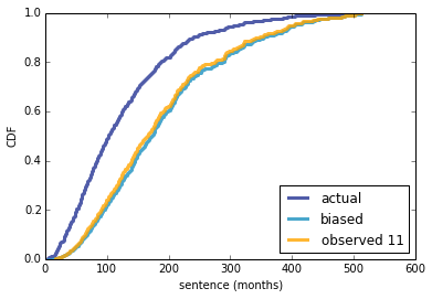
The observed distribution is almost as biased as what would be seen by an instantaneous observer. Even after 120 months (near the average sentence), the observed distribution is substantially biased:
 After 600 months (50 years!) the observed distribution nearly converges to the actual distribution.
 I conclude that during Kerman's 11 month sentence, she would have seen a biased sample of the distribution of sentences. Nevertheless, her observation — that many prisoners are serving long sentences that do not fit their crimes — is still valid, in my opinion.

About half of federal prisoners were convicted of drug crimes, according to this fact sheet from the US Sentencing Commission (USSC). In minimum security prisons, the proportion is higher, and in women's prisons, I would guess it is even higher. About 45% of federal prisoners were sentenced under mandatory minimum guidelines that sensible people would find shocking. And about a third of them had no prior criminal record, according to this report, also from the USSC.
In many cases, minor drug offenders are serving sentences much longer than sentences for serious violent crimes. For a list of heart-breaking examples, see these prisoner profiles at Families Against Mandatory Minimums.
Or watch this clip from Jon Oliver's Last Week Tonight:
When you are done being outraged, here are a few things to do:
1) Read more about Families Against Mandatory Minimums, write about them on social media, and consider making a donation (Charity Navigator gives them an excellent rating).
2) Another excellent source of information, and another group that deserves support, is the Prison Policy Initiative.
3) Then read the rest of this article, which points out that although Kerman's observations are fundamentally correct, her sampling process is biased in an interesting way.
The inspection paradoxIt turns out that Kerman is the victim not just of a criminal justice system that is out of control, but also of a statistical error called the inspection paradox. I wrote about it in Chapter 3 of Think Stats, where I called it the Class Size Paradox, using the example of average class size.
If you ask students how big their classes are, the average of their responses will be higher than the actual average, often substantially higher. And if you ask them how many children are in their families, the average of their responses will be higher than the average family size.
The problem is not the students, for once, but the sampling process. Large classes are overrepresented in the sample because in a large class there are more students to report a large class size. If there is a class with only one student, only one student will report that size.
And similarly with the number of children, large families are overrepresented and small families underrepresented; in fact, families with no children aren't represented at all.
The inspection paradox is an example of the Paradox Paradox, which is that a large majority of the things called paradoxes are not, actually, but just counter-intuitive truths. The apparent contradiction between the different averages is resolved when you realize that they are averages over different populations. One is the average in the population of classes; the other is the average in the population of student-class experiences.
Neither is right or wrong, but they are useful for different things. Teachers might care about the average size of the classes they teach; students might care more about the average of the classes they take.
Prison inspectionThe same effect occurs if you visit a prison. Suppose you pick a random day, choose a prisoner at random, and ask the length of her sentence. The response is more likely to be a long sentence than a short one, because a prisoner with a long sentence has a better chance of being sampled. For each sentence duration, x, suppose the fraction of convicts given that sentence is p(x). In that case the probability of observing someone with that sentence is proportional to x p(x).
Now imagine a different scenario: suppose you are serving an absurdly-long prison sentence, like 55 years for a minor drug offense. During that time you see prisoners with shorter sentences come and go, and if you keep track of their sentences, you get an unbiased view of the distribution of sentence lengths. So the probability of observing someone with sentence x is just p(x).
And that brings me to the question that occurred to me while I was reading Orange: what happens if you observe the system for a relatively short time, like Kerman's 11 months? Presumably the answer is somewhere between p(x) and x p(x). But where? And how does it depend on the length of the observer's sentence?
I tried for a little while to find an analytic answer for an arbitrary distribution of x. I didn't find one, and if there is one, I will be pleasantly surprised. But this is a case where analysis is hard (at least for me) and simulation is easy (at least for me).
This IPython notebook has the details, and here's a summary of the results.
ResultsTo model the distribution of sentences, I use random values from a gamma distribution, rounded to the nearest integer. All sentences are in units of months. I chose parameters that very roughly match the histogram of sentences reported by the USSC.
The following code generates a sample of sentences as observed by a series of random arrivals. The notebook explains how it works.
sentences = np.random.gamma(shape=2, scale=60, size=1000).astype(int)
releases = sentences.cumsum()arrivals = np.random.random_integers(1, releases[-1], 10000)prisoners = releases.searchsorted(arrivals)sample = sentences[prisoners]cdf2 = thinkstats2.Cdf(sample, label='biased')
The following figure shows the actual distribution of sentences (that is, the model I chose), and the biased distribution as would be seen by random arrivals:
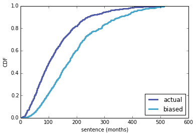 Due to the inspection paradox, we oversample long sentences. As expected, the sample mean is substantially higher than the actual mean, about 190 months compared to 120 months.
The following function simulates the observations of a person serving a sentence of t months. Again, the notebook explains how it works:
def simulate_sentence(sentences, t):
counter = Counter()
releases = sentences.cumsum()
last_release = releases[-1]
arrival = np.random.random_integers(1, max(sentences))
for i in range(arrival, last_release-t, 100):
first_prisoner = releases.searchsorted(i)
last_prisoner = releases.searchsorted(i t)
observed_sentences = sentences[first_prisoner:last_prisoner 1]
counter.update(observed_sentences)
print(sum(counter.values()))
return thinkstats2.Cdf(counter, label='observed %d' % t)
Here's the distribution of sentences as seen by someone serving 11 months, as Kerman did:

The observed distribution is almost as biased as what would be seen by an instantaneous observer. Even after 120 months (near the average sentence), the observed distribution is substantially biased:
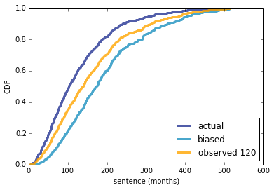 After 600 months (50 years!) the observed distribution nearly converges to the actual distribution.
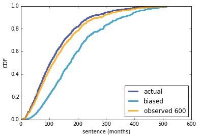 I conclude that during Kerman's 11 month sentence, she would have seen a biased sample of the distribution of sentences. Nevertheless, her observation — that many prisoners are serving long sentences that do not fit their crimes — is still valid, in my opinion.
Probably Overthinking It

Probably Overthinking It is a blog about data science, Bayesian Statistics, and occasional other topics.
- Allen B. Downey's profile
- 236 followers

