Nate Silver's Blog, page 174

The Clippers, Like Many NBA Teams, Have a Majority-Minority Fan Base

In light of the racist remarks attributed to Donald Sterling, the Los Angeles Clippers owner, on Monday we looked at the demographics of the NBA’s owners and players. Finding demographic information on NBA fans turns out to be more difficult.

In 2013, 47 percent of NBA head coaches and 81 percent of players were non-white. It’s likely that the majority of NBA fans are racial or ethnic minorities as well, according to our analysis. And the Clippers, which play in the cosmopolitan Los Angeles market, likely have among the most diverse fan bases in the league.

There’s no definitive resource for the demographics of the NBA fan base. Nor is there any one definition of a fan. Those who attend NBA games are undoubtedly different from those who watch the NBA on TV, or who follow the NBA on the Internet, or who buy NBA merchandise, or who emulate their favorite NBA stars in pick-up games.

But I did the best I could by averaging data from five sources: a Nielsen report on the demographics of NBA TV viewership; polls from Pew Research and the Public Religion Research Institute on Americans’ favorite sports; a Scarborough Research report on avid NBA fans, and a YouGov poll on which sports Americans follow regularly.

These sources provide estimates of how many Americans of different racial and ethnic groups follow the NBA as compared to the country as a whole. These tendencies can be expressed in the form of a multiplier. For example, the various surveys estimate that African-Americans follow the NBA at a multiple of somewhere between 2.2 and 3.3 times the national average. White Americans, by contrast, follow the NBA at rates between 0.6 and 0.9 times the national average, depending on the survey.

Estimates of NBA avidity among Hispanic Americans vary (perhaps, in part, because of the failure of some polling and research firms to conduct polls in Spanish). Hispanics overperform the rest of the U.S. population in NBA interest in some surveys, and underperform it in others. The consensus of the evidence, however, points toward Hispanics’ NBA avidity being about the same as the country as a whole. (For purposes of this analysis, I’ve taken “Hispanic” to be a non-overlapping category with both “white” and “black,” as most polls do. The U.S. Census Bureau, by contrast, treats Hispanic status as an ethnicity rather than a race – so in the census, someone can be both Hispanic and white, black or Asian.)

Only the Scarborough Research study contained a breakout for Asian-Americans. That study found that Asian-Americans are about 40 percent more likely to be avid NBA fans than the country as a whole.

We can estimate the racial and ethnic distribution of NBA fans by averaging the multiplier across the five studies, and then applying it to the overall U.S. population. I estimate — excluding those who identify themselves as Native American, or as belonging to “mixed” or “other” races — that about 46 percent of NBA fans are white, 31 percent are black, 7 percent are Asian-American and 16 percent are Hispanic. In other words, the league’s fan base appears to be majority-minority.

It’s also possible to come up with some crude estimates of the racial composition of fans for individual NBA teams. My process for doing this was as follows:

I used Nielsen estimates of the racial composition of the population in each of the United States’ 210 media markets;I used the frequency of Google searches for each NBA team in each media market as a proxy for its per-capita popularity;I multiplied each team’s Google search frequency in each media market by the population by race there, then summed the totals to produce an overall estimate of the racial distribution of its fans;I recalibrated the estimates to ensure that the whole matched the sum of the parts. In other words, I added or subtracted from the fans assigned from each racial group to each team such that the sum total matched my estimate of the overall distribution of NBA fandom throughout the country (e.g. 46 percent white, 31 percent black, and so forth). The estimates were weighted by the overall popularity of NBA teams, according to their number of Google searches.

I estimate that the team with the whitest fan base, at 65 percent white, is the Minnesota Timberwolves. The Minneapolis-St. Paul media market is 85 percent non-Hispanic white, according to our estimates. So Wolves’ fans are white relative to those elsewhere in the NBA. But they’re not so white compared to the media market the team calls home.

What about the Clippers? They aren’t all that popular in Los Angeles. But they hadn’t been all that popular anywhere in the country until they began to play well recently. So LA, and surrounding metropolitan areas, represent the bulk of the Clippers’ fan base. The Los Angeles media market is among the most diverse in the country: It’s only 36 percent non-Hispanic white, according to our estimates. I estimate the Clippers’ fan base to be 40 percent non-Hispanic white, 27 percent African-American, 22 percent Hispanic and 11 percent Asian-American. This implies that the Clippers have among the lowest proportions of white fans of any team in the NBA.

However, this estimate is crude. It’s based on the overall racial composition of NBA fans and the overall racial composition of various media markets. It won’t account for the historical relationship that each NBA franchise has with its fan base, or the different demographic groups that comprise that fan base.

Why LA Is Still a Lakers Town

Since Google began tracking search terms in 2004, people in the Los Angeles area have searched for the Lakers eight times more often than they’ve searched for the Clippers.

The gap has narrowed since the Clippers traded for Chris Paul in December 2011, but not by that much. The Lakers have received 3.6 times more search traffic from Angelenos since October, when the current NBA season started. This in a year in when the Lakers went 27-55 and the Clippers 57-25.

Having an owner like Donald Sterling, with his history of racist remarks and discriminatory business practices, won’t help the Clippers’ popularity (although it may spark more Google searches in the short term). And it’s not as if the team has been any good on the court under his ownership. Since the 1984-85 NBA season, when Sterling moved the Clippers to Los Angeles from San Diego, they are 582 games under .500, counting both the regular season and the playoffs. The Lakers are 772 games over .500 in the same period.

Lately, the Clippers have been better, but it will take them some time to catch up. Even if they go 57-25 every season (and break even in the playoffs), they would need until some point in the 2031-32 season to pull themselves over the .500 line.

Both Republicans And Democrats Have an Age Problem

The New York Times ran a long feature earlier this month claiming that the election of President Barack Obama in 2008 has done little to inspire young people to run for office. The article had some strong reporting but did not cite much statistical evidence. So here’s a simple question: Is the U.S. Congress getting younger?

No. The trend in recent years has been toward an older Congress. It’s gotten no better — and maybe a bit worse — under Obama.

We collected data from a variety of sources, including GovTrack.us, the Sunlight Foundation and The New York Times’ Congress API, on members of Congress since 1947. (We’ve posted our data compilation here.) The people who represent us are considerably older than the population as a whole. The average member of the current 113th Congress was 57.6 years old as of the start of the term on Jan. 3, 2013. This is close to the all-time high of 57.8 years, which was achieved in the 111th Congress, which came into office with Obama in 2009. By contrast, the average age was 53.0 in January 1993, when Bill Clinton took office, and 49.5 when Ronald Reagan did in 1981.

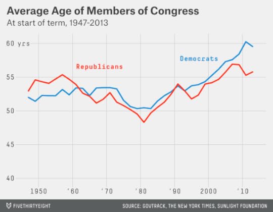
Democrats in Congress average 59.6 years old — older than Republicans, who are 55.8. Democrats have been older in each congressional term since the 104th Congress, which came into office after the Republicans’ “Contract With America” wave election of 1994. But the gap has widened in the current and previous Congresses, under Obama.

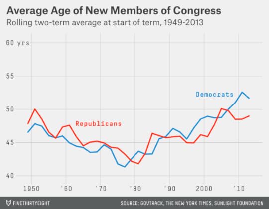
One might think that Republicans’ relative youth reflects years like 1994 and 2010, when the GOP won a huge number of seats. New members of Congress are typically younger than the incumbents they replace. Those serving for the first time in the 113th Congress were an average of 50.5 years old on Jan. 3, 2013, less than the average of 59.2 years for those members who also served in the previous Congress.

We can correct for this by taking the average age only among new members of Congress. Democrats are still older by this measure. Those Democrats serving for the first time in the past two Congresses were an average of 51.7 years old at the start of their terms, older than newly serving Republicans, who were 49.0.

This evidence might seem counterintuitive: Aren’t Democrats the party preferred by young voters? Partisan preferences of the electorate by age have varied over the years, but young voters have favored Democrats recently. In 2012, Obama won voters under the age 30 by 23 percentage points.

However, it would be a mistake to think of Democrats who run for Congress as representative of a random subset of Obama voters. When it comes to voting for president, many Americans are “closet partisans”  — they may label themselves as independents, or say they are only weakly affiliated with one of the parties, but they can be counted on to vote for the same party most of the time.

These soft partisans may engage in a relatively narrow scope of political activity. Usually they vote in even-numbered years, and sometimes they follow political news. But they’re unlikely to donate to campaigns or to volunteer for them. They may be more interested in the underlying issues — anything from gay marriage to gun rights — than in the candidates and parties themselves.

By contrast, those people who seek federal office are by definition deeply immersed in partisan politics. They’ll need to be strong supporters of their parties’ agendas in order to win their nominations, rather than to take more heterodox views.

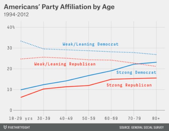
The General Social Survey, which has been conducted periodically since 1972, provides for a more nuanced view of Americans’ partisan leanings. We collected data from it dating back to 1994, which is roughly when Republicans began to be younger than Democrats in Congress.

In that survey, respondents are given a number of ways to label themselves, from independents without any partisan disposition to “strong Democrat” and “strong Republican.” It turns out that older Americans are much more likely to identify as strong partisans. Just 10 percent of those aged 18 to 29 identified themselves as strong Democrats in the sample. But the frequency increased with age, topping out at 23 percent for those aged 80 and older. The tendency to identify oneself as a “strong Republican” also increased with age, although the slope of the curve is a little flatter. By contrast, the number of soft partisans — Americans who identified themselves as weakly affiliated with one of the major parties — decreased with age.

We can frame this data another way: How old is the average “strong Democrat” or “strong Republican”? This is a better approximation of the pool from which congressional candidates may be drawn.

We’ve presented this data below, dating back to 1972, and aggregating different years of the General Social Survey under the president who was serving at the time. (Since the General Social Survey groups all respondents 89 or older into the same bucket, we used actuarial tables to estimate how old nonagenarian voters actually were.)

Republicans follow a v-shaped pattern: They became significantly younger under Reagan and George H.W. Bush as compared to under Richard Nixon and Gerald Ford. But they have grown older again since. The average “strong Republican” was 52.3 years old in the 2010 and 2012 versions of the survey.

The age of “strong Democrats” has been steadier, ranging between 48.6 and 49.9 years under each president from Nixon to George W. Bush. However, their average age has actually increased, to 50.7 years, under Obama.

The Americans who identify as strong partisans and who take the most active interest in politics are older still. In 2012, the General Social Survey asked Americans how informed they were about politics. Those who described themselves as strong Democrats and said they knew “quite a bit” or a “great deal” about politics were 52.7 years old, on average. The strong Republicans who said the same were 53.6 years old.

It’s very important to emphasize that these results do not imply that young people are uninterested in political affairs. Political movements ranging from Ron Paul’s campaigns in 2008 and 2012 to Occupy Wall Street to the push for gay marriage have been full of young people. However, these younger voters may be skeptical of the role played by the major parties. Disapproval rates of Congress remain near record highs. George W. Bush was unpopular for most of his second term, and Obama’s approval ratings have been underwater more often than not since 2010. These Americans may feel as though the major parties aren’t serving their interests very well.

They’ll often still vote. Youth turnout in presidential years has increased of late. But young people may not be interested in organizing the rest of their political activities under a partisan banner. Occupy Wall Street, for instance, was made up of a group of Americans who generally identified with the left, but not necessarily as Democrats.

Neither major party has seen its most politically active participants become younger since Obama took office. The question is whether this might become a vicious cycle; a Congress full of old people might serve the interests of younger Americans even less well.

To Find a Career Like Tim Duncan’s, We Have to Go Back to Kareem Abdul-Jabbar

Tim Duncan turns 38 on Friday. On Saturday, he’ll resume his quest for a fifth NBA championship when the San Antonio Spurs travel to Dallas to face the Mavericks in the third game of their first-round playoff series. Duncan is still an extremely effective player, in part because his masterful coach, Gregg Popovich, limits his minutes in the regular season. We might not have seen a career quite like his since Kareem Abdul-Jabbar.

Duncan has been a force since he entered the league at 21. In his debut season, 1997-98, he won the Rookie of the Year award and made the All-NBA team. The next year he was named NBA Finals MVP and won his first championship.

I wondered which other players in the NBA, and in the other major team sports, have had so much impact over their full professional lives. In other words, which of them were both very effective as young players and as old players?

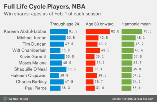
To study this for the NBA, I looked up the number of win shares each player has generated up to and including his age 24 season, and also from his age 33 season onward. (From this point forward, I’ll define an NBA player’s age-season by how old he was as of Feb. 1, as Basketball-Reference.com does.) Then I took the harmonic mean between the two figures. The harmonic mean differs from a regular average in that it tends toward the lower of a set of numbers. That will help us to identify players who were outstanding both when they were young and when they were old, as opposed to just one or the other.

Duncan generated 47.8 win shares through his age 24 season. That’s very good, especially considering that he stayed all four years at Wake Forest University before entering the league. But it’s still just the 17th-highest figure in NBA history. He’s also generated 40.2 win shares, and counting, since his age 33 season. That’s the 15th-highest figure in league history.

It’s having accomplished both of these things in the same career that makes Duncan so extraordinary. The harmonic mean between his early-career and late-career win share totals is 43.7. That’s the third-highest figure ever in the NBA.

You can probably guess the two players who rank ahead of Duncan. One is Michael Jordan, who achieved this feat despite retiring for his age 35 through age 37 seasons. (Jordan came back to play seasons with the Washington Wizards at 38 and 39.) But the player who laps the field, and who in many ways was the predecessor to Duncan, is Kareem Abdul-Jabbar.

Abdul-Jabbar played into his 40s. By win shares, he was the third-best old player in NBA history, after Karl Malone and John Stockton.

Those of you who are my age might only remember Old Kareem and his skyhooks and might not know what a phenom he was when he entered the league as Lew Alcindor. Abdul-Jabbar/Alcindor was the sixth-most productive young player in NBA history — despite, like Duncan, playing out his full college career. In his rookie season with the Milwaukee Bucks, he averaged 28.8 points and 14.5 rebounds per game. Two years later, at 24, he averaged 34.8 and 16.6.

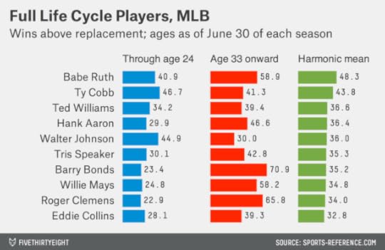
No player in the other major sports stands out so much from his competition. Babe Ruth is the top-ranking baseball player (counting his days as a pitcher and using wins above replacement; note that the systems we’re using for the various sports are not directly comparable to one another). Still, many of the all-time great baseball players have had extremely long careers. Ty Cobb ranks second and isn’t all that far behind Ruth.

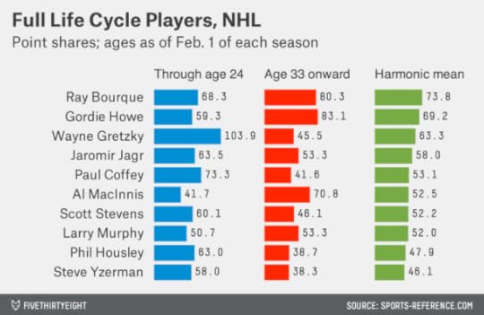
You might assume that the top NHL player by this standard absolutely must be Wayne Gretzky, or if not Gretzky then Gordie Howe. But it’s Ray Bourque. Gretzky was the best young player in NHL history by leaps and bounds, and Howe was the most productive old one. But Bourque had the best balance over his career, and he comes out slightly better when you take the harmonic mean of his point shares. I’m not sure that I totally buy that ranking — hockey analytics are behind those in baseball and basketball. But Gretzky was a somewhat specialized player late in his career. He notched tons of assists, but never ranked in the top 10 in goals in the NHL after his age 28 season, and he was limited defensively, with a -93 plus-minus from his age 33 season onward.

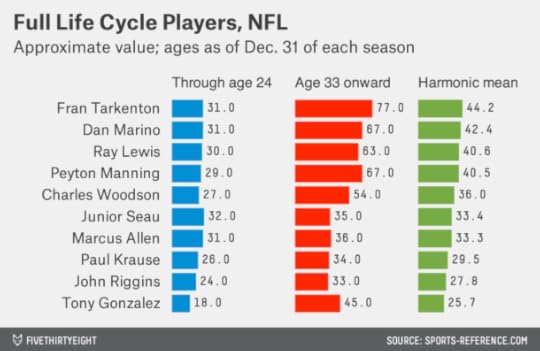
Last is the NFL, which is the least interesting of the leagues to evaluate in this way. That’s because NFL careers start late due to the league’s strictly enforced age limit and end early because of the wear and tear on the players. And it’s hard to measure what goes on in between and to compare players at different positions.

Still, according to Sports-Reference.com’s approximate value system, the closest thing the NFL has had to a player for all seasons is Fran Tarkenton. As a rookie, at age 21, Tarkenton was the principal quarterback for the expansion Minnesota Vikings. By 24, he led the Vikings to their first winning season, in 1964, and made his first Pro Bowl. After a stint with the New York Giants, he returned to Minnesota, and won an MVP award at age 35 and led the NFL in passing yards in his final season at age 38. Dan Marino, Ray Lewis and Peyton Manning rank next after Tarkenton. (Note that approximate value figures are incomplete for the 2013 season; I had to make an educated guess for how Charles Woodson and Tony Gonzalez performed last year according to the system.)

Manning could take over the top slot with one or two more good seasons. It seems like he should be ahead already. Approximate value is … approximate. And like the other measures, it doesn’t account for the post-season. I have trouble ranking Peyton Manning behind Fran Tarkenton in pretty much anything.

But I don’t have a problem with ranking Manning, or Duncan, behind Abdul-Jabbar, who won a national championship as a teenager at UCLA and an NBA title with the Los Angeles Lakers in his 40s. No player in American team sports has had a career quite like his.

To Find a Career Like Tim Duncan’s, We Have To Go Back To Kareem Abdul-Jabbar

Tim Duncan turns 38 on Friday. On Saturday, he’ll resume his quest for a fifth NBA championship when the San Antonio Spurs travel to Dallas to face the Mavericks in the third game of their first-round playoff series. Duncan is still an extremely effective player, in part because his masterful coach, Gregg Popovich, limits his minutes in the regular season. We might not have seen a career quite like his since Kareem Abdul-Jabbar.

Duncan has been a force since he entered the league at 21. In his debut season, 1997-98, he won the Rookie of the Year award and made the All-NBA team. The next year he was named NBA Finals MVP and won his first championship.

I wondered which other players in the NBA, and in the other major team sports, have had so much impact over their full professional lives. In other words, which of them were both very effective as young players and as old players?

To study this for the NBA, I looked up the number of win shares each player has generated up to and including his age 24 season, and also from his age 33 season onward. (From this point forward, I’ll define an NBA player’s age-season by how old he was as of Feb. 1, as Basketball-Reference.com does.) Then I took the harmonic mean between the two figures. The harmonic mean differs from a regular average in that it tends toward the lower of a set of numbers. That will help us to identify players who were outstanding both when they were young and when they were old, as opposed to just one or the other.

Duncan generated 47.8 win shares through his age 24 season. That’s very good, especially considering that he stayed all four years at Wake Forest University before entering the league. But it’s still just the 17th-highest figure in NBA history. He’s also generated 40.2 win shares, and counting, since his age 33 season. That’s the 15th-highest figure in league history.

It’s having accomplished both of these things in the same career that makes Duncan so extraordinary. The harmonic mean between his early-career and late-career win share totals is 43.7. That’s the third-highest figure ever in the NBA.

You can probably guess the two players who rank ahead of Duncan. One is Michael Jordan, who achieved this feat despite retiring for his age 35 through age 37 seasons. (Jordan came back to play seasons with the Washington Wizards at 38 and 39.) But the player who laps the field, and who in many ways was the predecessor to Duncan, is Kareem Abdul-Jabbar.

Abdul-Jabbar played into his 40s. By win shares, he was the third-best old player in NBA history, after Karl Malone and John Stockton.

Those of you who are my age might only remember Old Kareem and his skyhooks and might not know what a phenom he was when he entered the league as Lew Alcindor. Abdul-Jabbar/Alcindor was the sixth-most productive young player in NBA history — despite, like Duncan, playing out his full college career. In his rookie season with the Milwaukee Bucks, he averaged 28.8 points and 14.5 rebounds per game. Two years later, at 24, he averaged 34.8 and 16.6.

No player in the other major sports stands out so much from his competition. Babe Ruth is the top-ranking baseball player (counting his days as a pitcher and using wins above replacement; note that the systems we’re using for the various sports are not directly comparable to one another). Still, many of the all-time great baseball players have had extremely long careers. Ty Cobb ranks second and isn’t all that far behind Ruth.

You might assume that the top NHL player by this standard absolutely must be Wayne Gretzky, or if not Gretzky then Gordie Howe. But it’s Ray Bourque. Gretzky was the best young player in NHL history by leaps and bounds, and Howe was the most productive old one. But Bourque had the best balance over his career, and he comes out slightly better when you take the harmonic mean of his point shares. I’m not sure that I totally buy that ranking — hockey analytics are behind those in baseball and basketball. But Gretzky was a somewhat specialized player late in his career. He notched tons of assists, but never ranked in the top 10 in goals in the NHL after his age 28 season, and he was limited defensively, with a -93 plus-minus from his age 33 season onward.

Last is the NFL, which is the least interesting of the leagues to evaluate in this way. That’s because NFL careers start late due to the league’s strictly enforced age limit and end early because of the wear and tear on the players. And it’s hard to measure what goes on in between and to compare players at different positions.

Still, according to Sports-Reference.com’s approximate value system, the closest thing the NFL has had to a player for all seasons is Fran Tarkenton. As a rookie, at age 21, Tarkenton was the principal quarterback for the expansion Minnesota Vikings. By 24, he led the Vikings to their first winning season, in 1964, and made his first Pro Bowl. After a stint with the New York Giants, he returned to Minnesota, and won an MVP award at age 35 and led the NFL in passing yards in his final season at age 38. Dan Marino, Ray Lewis and Peyton Manning rank next after Tarkenton. (Note that approximate value figures are incomplete for the 2013 season; I had to make an educated guess for how Charles Woodson and Tony Gonzalez performed last year according to the system.)

Manning could take over the top slot with one or two more good seasons. It seems like he should be ahead already. Approximate value is … approximate. And like the other measures, it doesn’t account for the post-season. I have trouble ranking Peyton Manning behind Fran Tarkenton in pretty much anything.

But I don’t have a problem with ranking Manning, or Duncan, behind Abdul-Jabbar, who won a national championship as a teenager at UCLA and an NBA title with the Los Angeles Lakers in his 40s. No player in American team sports has had a career quite like his.

Stop Betting Against Gregg Popovich

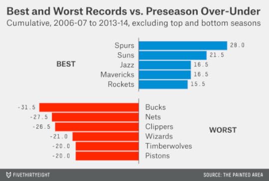
The San Antonio Spurs’ Gregg Popovich won his third NBA Coach of the Year Award on Tuesday. To an extent, these awards are about which coach most exceeds expectations: They’re the opposite of coach firings, which are better predicted by a coach’s performance relative to preseason Las Vegas over-under lines than by his win-loss record. Popovich’s Spurs won 62 games in the regular season — more than the 55.5 wins Vegas predicted. That’s reasonably impressive, but nothing as compared to the Phoenix Suns’ Jeff Hornacek, who finished second in the balloting after winning 27 more games than Vegas anticipated.

What’s more amazing is how Popovich and the Spurs keep beating even consistently high expectations. From the 2006-07 through the 2013-14 seasons, the Spurs have outperformed their preseason over-under lines by a cumulative 35.5 games. That is the second-best total in the NBA, after the Suns, who were boosted by their extraordinary performance this year. It comes despite the fact that the Spurs have been projected to win an average of 53.2 games during this period, the highest figure in the league over this stretch. (These figures include the labor-shortened 2011-12 season, for which I’ve prorated totals to 82 games.)

Popovich took over as coach of the Spurs early in the 1996-97 season. I wanted to evaluate his performance against the preseason over-under line further back, but I couldn’t find reliable numbers. However, there are records of how the Spurs performed against the point spread for individual games dating to the beginning of Popovich’s tenure. Popovich has done just as impressively by this benchmark.

The table below lists the Spurs’ win-loss record against the point spread since Popovich took over as coach. It includes regular-season and playoff games, although a handful of regular-season games from his earliest seasons are missing. In total, in the games for which we have data, Popovich has 843 wins, 728 losses and 32 pushes against the point spread. That’s a 53.7 percent winning percentage, ignoring pushes, a win rate that all but the best sports bettors in the world would have trouble sustaining.

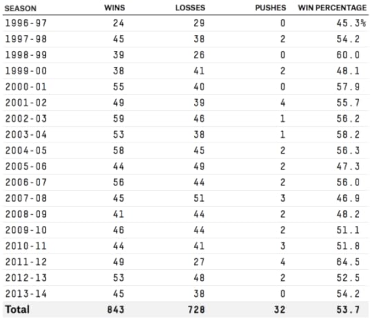
How plausible is it that Popovich has just gotten lucky? We can check this by means of a binomial distribution. If Popovich were just a .500 coach against the point spread, the probability that he’d achieve a 843-728 record or better against it is just 0.17 percent. In other words, this is an awful lot of games, and Pop has done awfully well. It’s likely that there’s something going on — something the betting public has been missing. (And it’s something that it has been missing continually; Popovich’s edge has not abated recently. The Spurs’ record against the point spread over the past five seasons is 54.5 percent.)

I looked at a few theories. For instance, could the Spurs’ excellent record against the point spread reflect a bias against small-market teams, rather than anything about Popovich? This may represent a tiny part of it; there’s a modest inverse correlation between teams’ performance against the point spread and their market size (meaning that teams in smaller markets tend to do a bit better against the spread). But the effect is small; it’s enough to account for the Spurs winning 50.4 percent of their games against the point spread, but nothing like 53.7 percent.

Another theory: Perhaps the Spurs tend to perform poorly early in the season — lowering bettors’ expectations — and then improve as Popovich determines the strengths of his roster and adjusts? That doesn’t quite pan out. Since the 1997-98 season, the Spurs are 53.5 percent against the point spread in the first 20 games of the regular season, about the same as their performance overall. (They have done somewhat better against the point spread — a 55.9 percent winning percentage — during the playoffs.)

Maybe there’s something odd about the Spurs’ point distribution? If they took an unusual number of blowout losses for a good team — say, games when Popovich was resting his starters — that could artificially lower their average margin of victory and lead bettors to underrate them in other matchups.

However, the Spurs’ point distribution appears to be relatively normal (both in the common-language and mathematical senses of the term) and relatively symmetrical about their average margin of victory. The Spurs have been somewhat less likely to win or lose games by exactly one point than the normal distribution would predict, but this is true of all NBA teams, largely as a result of late fouling. I don’t want to completely dismiss these explanations: How NBA teams manage endgame situations is something that can affect their scoring distribution and performance against the point spread quite a bit. But there’s nothing obvious that jumps out about the Spurs. Nor have they won more games than would be expected based on their overall scoring margin.

Another tempting explanation is that the Spurs, under Popovich, have great “intangibles” that bettors underrate. Undoubtedly, Popovich (like Tim Duncan) is a great leader. But eventually those intangibles should manifest themselves in the form of the Spurs winning more games than they otherwise would, and bettors should see the results and adjust accordingly. Furthermore, Popovich and the Spurs have a reputation for strong coaching and veteran leadership that could be recognized by the betting market. For many years, Popovich has ranked at or near the top when NBA general managers were asked to rank the top coaches.

In the absence of an explanation, I was curious about another data point. The coach I think of as being most Pop-like is Bill Belichick of the NFL’s New England Patriots. Like Popovich, Belichick seems to have a preternatural ability to make the most of his circumstances — he got 11 wins out of Matt Cassel! Like Popovich, Belichick has a reputation as a great and ruthless tactician.

Also like Popovich, Belichick has done quite well against the point spread. He’s 179-144-9 against it lifetime (a 55.4 percent winning percentage, ignoring pushes), counting his time as coach of the Cleveland Browns. (He’s 138-106-6 against the point spread, a 56.6 percent winning percentage, as coach of the Patriots.)

I’m aware of the risk of confirmation bias here. If you seek out coaches who have a reputation for exceeding expectations, you’re likely to find expectations exceeded in all sorts of data, including their performance against the point spread. Nevertheless, it’s worth asking whether there is something about coaches like Popovich and Belichick that leads them to outperform bettors’ expectations.

I don’t have a sexy answer. Nor am I sure that there is a sexy answer. It may be that Popovich’s strong performance against the point spread reflects a little bit of luck, a little bit of small-market bias, a little bit of something funny about how the Spurs manage endgame situations — along with a healthy dose of selection bias in our decision to examine his record (and not that of other coaches) after the fact.

But I have a romantic notion of what could be going on.

What you might say about Popovich is that he’s been uniquely able to stave off regression to the mean. He adopts tactics and strategies to suit his situation; he stays one step ahead of his opponents. Under Popovich, the Spurs have succeed as an old team and as a young team, and as a fast-paced team and a slow-paced team. There isn’t much gimmicky about Popovich.

Perhaps in staying one step ahead of his opponents, he has stayed one step ahead of Las Vegas. The reason it’s hard to succeed in sports betting, or in any other market-based activity, is not just that markets are reasonably efficient to begin with. It’s also that when you’ve identified a historical tendency worth exploiting, other participants in the market may have found it as well. You may have an advantage for a while, but it will evaporate soon. Or, like in the game rock-paper-scissors, your opponents will exploit you for trying to exploit them.

But what if your advantage is not in finding one particular loophole in the market, but in having the aptitude to continually come up with new advantages? Before your opponent has identified a counter to your tactic, you’re on to the next tactic. Great poker players have this skill: They have a sense for when a particular tactic in a particular situation has gone from being underutilized to overutilized in the poker “market.” They’ve adjusted a moment before everyone else.

My romantic notion — my intuition — is that the way coaches like Popovich and Belichick exploit edges in their games is pretty similar to how sports bettors exploit edges in theirs. So the fact that opponents have never caught up with Popovich and Belichick may have something to do with why betting markets haven’t either. I do know that I wouldn’t bet against Popovich or Belichick. And I wouldn’t want to play poker against them.

In the NBA, It’s Not Whether You Win or Lose, It’s Whether You Beat Vegas

It was the age of foolishness. It was the summer of trading three draft picks for Andrea Bargnani. It was the autumn of J.R. Smith being suspended for marijuana possession. It was the winter of disparaging the shot clock.

It was the New York Knicks’ 2013-14 season. So when Mike Woodson was fired as the coach of the Knicks on a warm, spring day in Gotham Monday, New York breathed a sigh of relief.

But Woodson’s problem wasn’t just that the Knicks were bad. The Knicks are usually bad. Woodson’s problem was that the Knicks — for a change — were expected to be good. They’d won 54 games and gone to the Eastern Conference semifinals the year before. Preseason over-under lines pegged their win total at 49.5 games. When my ESPN colleague Kevin Pelton, through his SCHOENE system, instead projected the Knicks to win 37 games, his projection threatened to turn Knickerblogger, the eminently sane and stats-friendly blog, into the basketball version of “unskewed polls.”

The Knicks went 37 and 45.

In the NBA, where about 30 percent of the league turns its head coach over every season, these expectations matter as much as reality. I mean that literally: Las Vegas’s preseason over-under lines predict coach turnover just as well as actual wins and losses do.

I went back and collected preseason over-under lines dating back to the 2006-07 season. I compared them to each team’s actual record during the regular season. Then I ran a logistic regression analysis. The dependent variable is whether the team kept the same head coach from the start of that regular season to the next one. Here are the results:

The regression output contains two variables: exp_w (the number of games a team was expected to win, per Las Vegas) and act_w (actual wins). For the 2011-12 NBA season, which was shortened by a player lockout, I’ve prorated both totals to 82 games.

You may notice that the coefficient on each variable is almost identical, though they have opposite signs. What that means is that an expected win hurts a coach about as much as an actual win helps him.

The graph below provides an illustration of this, and measures the probability of a coaching change under two scenarios: a team (like this year’s Sacramento Kings) that was expected to win 30 games, and a team (like the Knicks) that was expected to win 50. If the projected 30-win team wins 35 games, just slightly better than expectations, its probability of a coaching change is only about 17 percent. If the projected 50-win team wins 45 games, just slightly worse than expectations, the probability is 37 percent instead.

Lest this seem too abstract, I’ve compiled a list of all teams since the 2006-07 season that underperformed their over-under line by 10 games or more. There are 33 of these. Here’s what happened to their coaches:

Nine of them were fired during the season;Nine of them were fired after the season;One of them resigned during the season;Two of them resigned after the season;Two of them, Larry Drew of the Milwaukee Bucks and Brian Shaw of the Denver Nuggets, just completed their seasons and have yet to learn their fates;The other 10 kept their jobs, although five of them were fired during or after their following season.

Other factors also affect a coach’s odds of being fired. Deep playoff runs help coaches. First-year coaches sometimes get mulligans and are less likely to be fired. We’ll save that discussion for another post, however.

The lesson is simple: A coach is not long for his job when expectations run wild, as they often do in New York. With the benefit of hindsight, it now seems likely that Woodson’s Knicks overachieved in the 2012-13 season. That only made it harder for him to keep his job this year.

Which Cities Sleep in, and Which Get to Work Early

I’m not a morning person, so I appreciate living in New York. The workday here starts later than in any other American city, and about half an hour later than in the U.S. as a whole.

A decade or so ago, when I was a consultant living in Chicago, I didn’t have it so easy. Work in Chicago begins a little earlier than in New York — about 20 minutes earlier, relative to the local time zone. My bosses nevertheless tolerated me rolling into the office at a bit past 9 a.m. But sometimes I’d travel to cities such as St. Louis and Omaha, Neb., to visit clients. Meetings as early as 6 or 7 a.m. were not uncommon; I was “relieved” from one project after a client caught me nodding off in a meeting.

How much do American cities differ in when they begin work? The Census Bureau collects data on this through the American Community Survey. This data isn’t especially user-friendly, but I figured out the median time Americans begin their workday in each metro area. All the figures that I’ll describe here refer to the location of work — not the location of residence for the workers — since some Americans commute between metro areas for their jobs. These figures also don’t include the growing number of Americans who work from home. All times are local.

As I mentioned, New Yorkers get to work late — at least on a relative basis. The median worker in the New York metropolitan area begins her workday at 8:24 a.m. There’s a buffer of about an hour on either side: 25 percent of the workforce has arrived by 7:28 a.m., while 75 percent has gotten in by 9:32.

The 20 most nocturnal metro areas, by the median time of arrival at work, are as follows:

These cities break down into three rough categories. First are those like New York, San Francisco and Boston, which are home to a lot of young, creative professionals. Next are college towns such as Ithaca, N.Y. (Cornell University); Lawrence, Kan. (the University of Kansas); and Logan, Utah (Utah State University). Finally are cities such as Atlantic City, N.J., Orlando, Fla., and Miami, whose economies are associated with recreation, tourism and gambling. A quarter of the workforce in Atlantic City doesn’t begin its workday until 11:26 a.m. or after.

The metro area with the earliest workday is Hinesville, Ga. The median worker there arrives at work at 7:01 a.m. There’s a good chance she is in the military; the Hinesville area includes Fort Stewart and the Army’s 3rd Infantry Division. Military metros account for a number of the earliest-to-work communities, including Killeen, Texas (Fort Hood), and Jacksonville, N.C. (Camp Lejeune). Many of the other early-arriving metros, such as Bakersfield, Calif., rely on farming and agriculture to generate income.

One exception is Honolulu, where the median workday begins at 7:29 a.m. Presumably, some workers there are trying coordinate with the U.S. mainland. This is not true of Anchorage, Alaska, however, where the median workday starts at 7:57, two minutes after the U.S. median of 7:55. While Anchorage is four hours behind the East Coast, its northerly location presents another constraint for some workers: sunrise there doesn’t occur until after 8 a.m. for five months out of the year.

What about those mid-size Midwestern metros, such as St. Louis? Work in St. Louis indeed begins begins relatively early, at 7:50. In Omaha, the median workday starts at 7:48. Kansas City, Mo. (7:51), Milwaukee (7:51) — also places on my consulting itinerary — likewise start their workday just slightly earlier than the U.S. median.

But the majority of highly populous metro areas begin working a little later than the rest of the country. (The chart below depicts the schedule for the 35 metro areas with the largest number of workers.) Washington, D.C., starts work at a median time of 8:07 (although it is prompt: three-quarters of the workforce is in by 9:14). The median worker in Los Angeles begins at 8:05; in Atlanta, at 8:03; in Chicago, at 8:02.

In general, however, the workday schedule is dictated more by the type of work than the location. The earliest-arriving quartile of the workforce in the New York metro has begun work by 7:28 a.m. — quite a bit sooner than the the latest-arriving quartile in Hinesville, which starts work at 8:06. Some of us New Yorkers appreciate our extra half-hour of sleep. But if you’re an early bird or a night owl and want a work schedule that matches your metabolism, changing jobs is a better strategy than changing cities.

Fly Early, Arrive On-Time

On Friday, I woke up at 4:45 a.m. to catch a flight home from Toronto. I’m not a morning person, and I forgot which airline I was flying. I went to the wrong terminal. I checked in late. I forgot that U.S. customs is on the Canadian side of the border. I was bumped from the flight. Fortunately, I made it to the gate with a few minutes to spare and was allowed to board as a standby passenger.

So the risk of human error may be higher early in the morning. But it’s the best time to fly if you want to minimize your time in the transit system.

The Bureau of Transportation Statistics keeps on-time data on every domestic flight flown by the 14 largest U.S.-based airlines. I collected summary data for the more than 6 million flights in the database in 2013 and organized them in one-hour blocks by their scheduled hour of departure (for instance, 10:00 a.m. to 10:59 a.m.). Then I looked at how many minutes late the flights arrived on average.

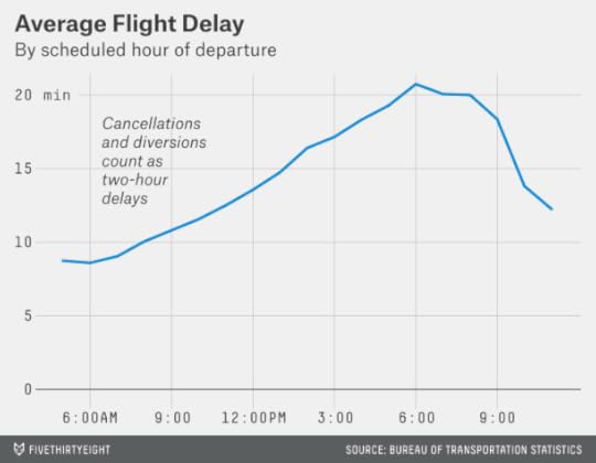
A few notes on this procedure: As should be clear, I prefer to look at delays in terms of time lost rather than a binary definition of arriving late or on time. (A 20-minute delay is nothing compared to a whole afternoon spent in transit hell.) I counted diverted and cancelled flights as equivalent to 120-minute delays. Some versions of the BTS data assign a flight negative minutes if it arrives early; I used a version where the minimum delay is 0 minutes instead.

The best time to fly is between 6 and 7 in the morning. Flights scheduled to depart in that window arrived just 8.6 minutes late on average. Flights leaving before 6, or between 7 and 8, are nearly as good.

But delay times build from there. Through the rest of the morning and the afternoon, for every hour later you depart you can expect an extra minute of delays. Delay times peak at 20.7 minutes — more than twice as long as for early-morning flights — in the block between 6 and 7 p.m. They remain at 20-plus minutes through the 9 p.m. hour.

Very late flights — those scheduled to leave at 10 p.m. or later — are much better. But it’s hard to find these, especially on the East Coast. Late flights represent only 2 percent of scheduled domestic departures.

What causes the accumulation of delays? The BTS data breaks delays down into five categories: aviation system delays, severe weather delays, late-arriving aircraft, security delays and carrier delays (such as those caused by mechanical or crew problems). Here’s the share of delay minutes each type of delay was responsible for:

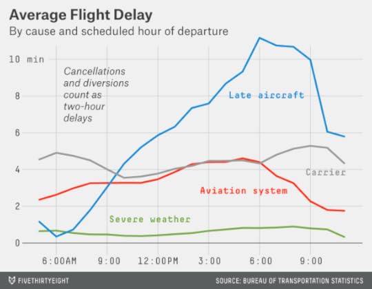
Late-arriving aircraft account for the bulk of the difference in the timing of delays. Ever have one of those days when you’re 10 minutes late to your first appointment and never make up the time? Airplanes are the same way. Early in the morning, almost all of them are in position from the previous evening. But there isn’t much slack. Once they’re late, their schedule may be off for the rest of the day.

Aviation system delays peak in the mid-to-late afternoon, when the transit system is at its fullest capacity. (The combined number of arrivals plus departures is highest between 4 and 5 p.m.) Weather-related delays are highest between 3 and 11 p.m., when thunderstorms are more likely to form. (These definitions are a little fuzzy: For instance, delays caused by moderately bad weather rather than severe weather are often classified as aviation system delays since they would theoretically be avoidable if the system was getting everything else right.)

Carrier delays are more or less constant throughout the day. Security delays constitute just 0.1 percent of the total — they’re too negligible to plot on the chart, and don’t much affect the best timing for your flight.

Perhaps these differences seem too small to be worth worrying about; a flight scheduled to depart at 10 a.m. is only 2.5 minutes more delayed on average than one that leaves at 7 a.m. But — based on my frequent travels — there are some other advantages to early flights that we haven’t yet accounted for.

Traffic can be much better when getting to the airport. Some airports have shorter security lines early in the morning (there are exceptions). Well-trained crews usually keep cabin announcements and other distractions to a minimum on very early flights, so it can be a lot easier to fall back asleep.

And if you’re like I am in the morning and miss your flight, you’ll be first in the queue for the rest of the day.

Why a Plan to Circumvent the Electoral College Is Probably Doomed

New York this week became the 10th state (plus D.C.) to join the National Popular Vote Interstate Compact. The compact represents a clever workaround to the Electoral College. By signing on, states agree they will award their electoral votes to the winner of the national popular vote (for example, New York would have given its electoral votes to George W. Bush in 2004). However, the measure will only be triggered once states accounting for a majority of electoral votes have joined.

There are 538 electoral votes (hence the name of this website), so a majority is 270. The compact’s signatories, so far, total 165 electoral votes. That represents a lot of progress since Maryland, with its 10 electoral votes, became the first state to join the compact in 2007.

Here’s the problem: All the states to have joined so far are very blue. Until some purple states and red states sign on, the compact has little in the way of territory to conquer.

As the chart below indicates, the relationship between whether a state has joined the compact and how it voted in 2012 is nearly 1-to-1. The seven states where President Obama won by the widest margins, along with D.C., have joined. So have three others — New Jersey, Illinois and Washington — where Obama won by at least 15 percentage points. But none below that threshold have done so.

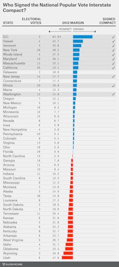
Perhaps the compact can get Delaware, Connecticut and Maine to join, where Obama also won by 15 percentage points or more. But they account for only 14 total electoral votes (and Maine already has a unique way of apportioning electoral votes). Oregon and New Mexico also re-elected Obama by double-digit margins — and those two states have become increasingly off-limits to Republican presidential candidates — but have just 12 electoral votes between them.

After that, you get into states such as Michigan and Minnesota, which are blue-leaning but that receive plenty of attention from presidential campaigns. Their votes might not be quite as influential in the Electoral College as the campaigns presume — a Democrat who lost Minnesota would probably be in too much trouble elsewhere to cobble together a 270-vote majority. Still, they receive an influx of media dollars and political pandering every four years, and probably have little incentive to bite the hand that feeds them.

Soon after comes outright swing states, such as Ohio, New Hampshire and Colorado. These states, along with Florida, Virginia, Nevada, Iowa, Wisconsin and Pennsylvania, collectively had a 98.6 percent chance of determining the Electoral College winner in 2012, according to the FiveThirtyEight tipping-point index as it was calculated on election morning. In other words, these nine states are 70 times more powerful than the other 41 (which collectively had a 1.4 percent chance of determining the winner) combined. That’s part of the reason so many Americans object to the Electoral College. But states whose voters have a disproportionate amount of influence may be in no mood to give it up.

Finally, there are the solidly red states, from Georgia to Utah; all the solidly red states together have 191 electoral votes. To advance further, the compact will need to collect some signatories from this group.

In theory, states that want a Republican in the White House might have a lot of incentive to join the compact. That’s because in the 2008 and 2012 elections, the Electoral College worked to Democrats’ benefit. States closest to the tipping point, such as Colorado, voted for Obama by a slightly wider margin than the nation as a whole. That implies that if there had been a uniform swing against Obama and he lost the national popular vote, he could have still won the Electoral College by eking out a victory in these states.

Could the red states come around? Perhaps. Despite Democrats’ painful memories of Al Gore’s Electoral College loss in 2000, Republican voters are nearly as likely to support ending the Electoral College (61 percent of them would vote to do away with it as compared to 66 percent of Democrats, according to a Gallup poll last year). But Republican legislators in those states evidently feel differently, or perhaps have calculated that the Democrats’ Electoral College advantage in 2008 and 2012 was an anomaly that will soon fade.

If Utah, Texas and similar states do begin signing onto the compact, what signal might that send to the blue states? Might legislators in Vermont and Maryland suddenly decide they agree with Alexander Hamilton’s position on the Electoral College after all?

My personal view is that the Electoral College should be abolished (even if that means we’d have to change the name of this website). But based on the signatories to the compact, blue and red states seem to think of it as a zero-sum game. And the purple states, which might otherwise swing the balance, have the least incentive of all to sign on.