Menzie David Chinn's Blog, page 3

Never Were Truer Words Said

“I am the king of debt. I do love debt. I love debt.” -Donald J. Trump, May 2016 (WaPo)

The Committee for a Responsible Federal Budget has released its score of the Presidential candidates’ plans. Here is the trajectory of Federal debt under the two plans.

Full report here.

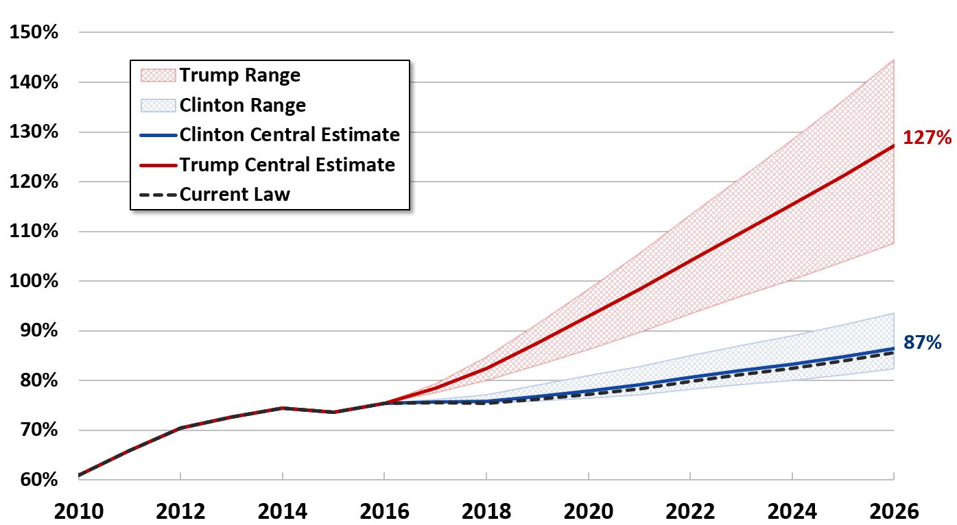
Increases in debt are not always a bad thing, particularly in times of economic slack, if the debt accumulation is driven by stimulative fiscal policy. But a 40 percentage points of GDP increase seems unlikely to be a positive outcome.

Guest Contribution: “Trump Jr.’s Pants-on-Fire Allegation of Manipulated Jobs Numbers”

Today, we present a guest post written by Jeffrey Frankel, Harpel Professor at Harvard’s Kennedy School of Government, and formerly a member of the White House Council of Economic Advisers.

When interviewed about the unemployment numbers, which have fallen steadily since 2010, Donald Trump Jr., replied “These are artificial numbers. These are numbers that are massaged to make the existing economy look good, to make this administration look good when, in fact, it’s a total disaster.” PolitiFact asked a variety of experts about the quote. Their bottom line: the quote from the younger Trump was a “Pants on Fire” lie. The truth is that presidents don’t and can’t manipulate the jobs numbers. No White House has even tried — at least not since Richard Nixon made a heavy-handed attempt in 1971 to interfere with BLS staffing. After that, extra firewalls were put in place.

Here is my own full response to PolitiFact’s question regarding the Trump claim:

The statement is 100% false. The employment numbers come from the Bureau of Labor Statistics (part of the Labor Department). In this administration, like every administration, those who produce the employment statistics are long-time nonpolitical professionals. The Secretary of Labor does not even know what the numbers are going to be when they are announced every month (the morning of the first Friday of the month).

Allegations that the official government numbers understate unemployment are sometimes based on a claim that some higher measure (which, for example, includes discouraged workers who have given up looking for a job, or part-time workers), should be used in place of the ones that get the most attention in the press. But these other measures are also made publicly available by the BLS and the press is free to write about them as much as they want.

The important thing, of course, is to be consistent across time in which measure you use. It wouldn’t be right to switch from looking at the conventional rate to a measure that includes discouraged workers just because you don’t like the incumbent president and want to make things look bad for him.

UK Yield Curve Flattening: “Nothing to do with Brexit”?

In response to this post, a reader asserts:

“[UK] Yield curve has been on a slide since 2010. Nothing to do with Brexit.

Check out global yield curve, looks similar to UK in that it has been on the slide for years as well.

It’s true yield curves have been flattening (as noted in this post). However, it is an empirical question whether the UK yield curve flattened more than others, upon the Brexit vote. Figure 1 compares the change in 10 year-3 month spreads from 18 June (before the vote) to today (July 25).

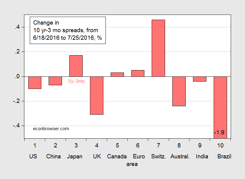
Figure 1: Change in the ten year-three month term spread (blue bars), from 18 June to 25 July 2016. China observation is Five year-three month term spread. Euro ten year rate is for Germany. Source: Economist, and author’s calculations.

If it’s not obvious, the UK experiences a bigger flattening than any other country in the sample, save Brazil. I don’t think it’s implausible it has something to do with Brexit.

Tracking US GDP ex.-Government

Political Calculations makes some more ([1], [2]) elementary errors with chained quantities, to arrive at incorrect — and misleading — measures of real GDP excluding government consumption and investment.

First, here is the figure that Political Calculations displays:

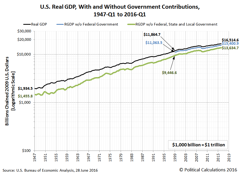
The real GDP ex-government was apparently calculated by simply subtracting Chain weighted government consumption and investment from Chain weighted GDP. (I verified this point by doing the subtraction myself, and matched his 2016Q1 figure.)

As is well known by professional economists, one cannot simply subtract one Chain-weighted measure from another, unless one is working with the reference period (i.e., looking only at 2009 values when the units are expressed in 2009 dollars.) Otherwise, one needs to use some sort of approximation method, such as this one.

Below is the correctly calculated series (in red) as compared to the incorrectly calculated (green) by Political Calculations.

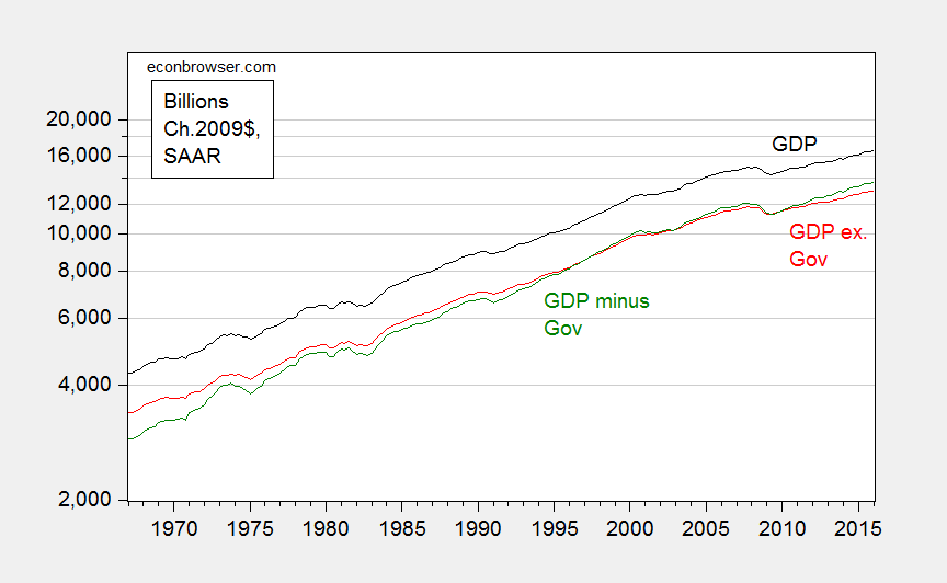
Figure 1: GDP (black), simple arithmetic subtraction of government consumption and investment from GDP (green), and Törnqvist approximation for GDP ex.-government consumption and investment (red), all in billions of Chained 2009$. Source: BEA 2016Q1 3rd release, and author’s calculations.

The error looks small in the graph, partly due to the log scale. In reality, the deviation is substantial, 4.9% (log terms) in 2016Q1. In other words, last quarter, actual ex.-gov GDP was 4.9% lower than what Political Calculations had asserted.

One might be tempted to conclude that if one examined data around the reference year (2009), there’d be little problem along all dimensions. This temptation should be resisted; for instance, calculating contributions to GDP growth using the simple-subtraction method would lead to very different inferences than if one used the correct measure. This is shown in Figure 2.

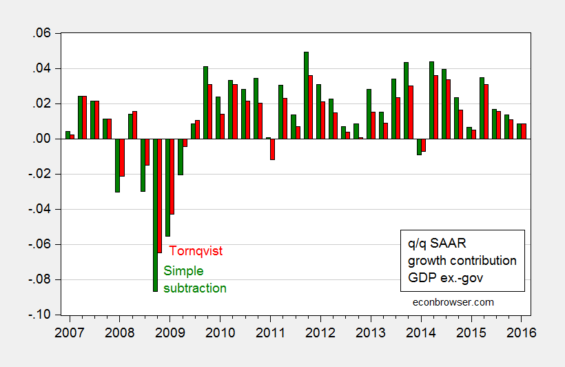
Figure 2: Quarter on quarter contribution of real GDP ex.-government consumption and investment to real GDP growth (red), and contribution of simple subtraction of government consumption and investment from GDP (green), at annualized rates, in percentage points. Source: BEA 2016Q1 3rd release, and author’s calculations.

In 2009Q1, non-government GDP was contributing -5.5 percentage points using the incorrect measure, and -4.3 percentage points (q/q SAAR) using the correct. The difference is even more stark moving to 2008Q4: 8.7 percentage points versus 6.5 percentage points.

On a related note, Political Calculations also makes a methodologically similar error in this post, as discussed here.

Heckuva Job, Nigel!

UK PMI collapses. Term spread moves toward inversion.

From yesterday’s FT:

A special edition of the purchasing managers’ index (PMI) – a well-regarded survey of activity produced by research group Markit – has been published to provide a picture of how the UK economy has fared after the referendum. The picture is not pretty.

The PMI survey for Britain’s powerhouse services sector – which accounts for nearly 80 per cent of the economy – has dropped to a seven year low of 47.4 for July from 52.3 at the June survey. Any reading below 50 indicates contraction. The outcome was far lower than economists’ forecast of a reading of 48.8.

Here’s the relevant graph.

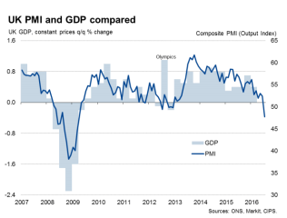
Source: “UK economy suffered ‘dramatic deterioration’ after Brexit vote – Markit,” FT, 22 July 2016.

The yield curve has not yet inverted.

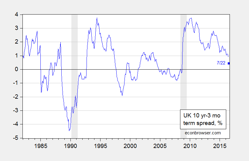
Figure 1: Ten year minus three month UK Treasury spread. July observation for 7/22. UK recession dates shaded gray. Source: BoE, Economist, Wikipedia, accessed 7/23.

Note that, as discussed in this post, most of the flattening of the yield curve has been due to a falling long yield, rather than a rising short rate.

While the yield curve does not appear to be a reliable indicator of recessions in the UK (as defined by ECRI), there is a statistically significant correlation between yield curve and (real time measures of) GDP growth over the subsequent 4 quarters (see Chinn and Kucko, 2015).

Δyt+4 = 1.43 + 0.47spreadt + ut+4

Adj-R2 = 0.14, N = 104, 1987Q3-2013Q2. bold denotes significant at the 5% msl, using HAC robust standard errors.

A drop in the spread of about 0.5 (that’s the drop in the ten year since the Brexit vote) implies about a 0.25 deceleration in GDP growth.

Wisconsin Employment: Five and a Half Years of Governor Walker

Wisconsin nonfarm payroll (NFP) employment is 63.2 thousand below what historical correlations with national employment would imply.

I use the observed relationship between US and Wisconsin nonfarm payroll employment over the 1994M01-2009M06 (NBER recession trough) period to construct a counterfactual for the 2009M07-2016M06 period, where ex post realizations of US NFP employment are incorporated (see this post for discussion). This leads to Figure 1.

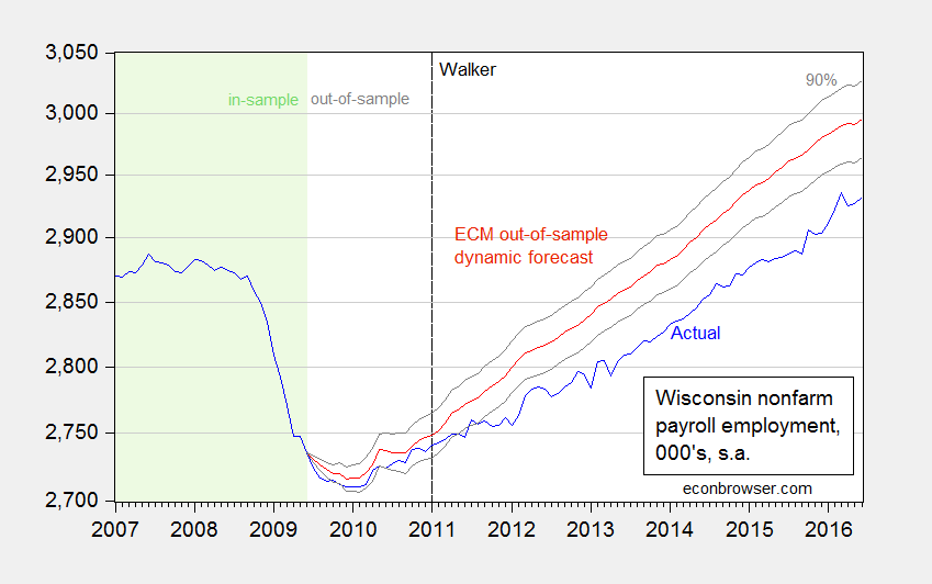
Figure 1: Wisconsin nonfarm payroll employment (blue), and forecasted (red), and 90% prediction interval (gray lines). Light green shaded area denotes in-sample data. Log scale on vertical axis. Source: BLS, and author’s calculations.

The Department of Workforce Development press release trumpets the 10,900 addition in private NFP in June. Tables indicate that May employment was revised down 6,300, which kinda takes off the gloss.

And if anybody was keeping track, we are over 47,000 jobs below the promised level of 250,000 new jobs by January 2015.

“Central Banks at a Crossroads: What Can We Learn from History?”

That’s the title of a book commissioned by the Norges Bank on the bicentennial of the Bank’s founding, and edited by Michael D. Bordo, Øyvind Eitrheim, Marc Flandreau and Jan F. Qvigstad (published by Cambridge University Press). Here’s the table of contents:

Preface

Michael D. Bordo, Øyvind Eitrheim, Marc Flandreau,

and Jan F. Qvigstad

1 Introduction

Michael D. Bordo, Øyvind Eitrheim, Marc Flandreau,

and Jan F. Qvigstad

2 The Descent of Central Banks (1400–1815)

William Roberds and François R. Velde

3 Central Bank Credibility: An Historical and Quantitative Exploration

Michael D. Bordo and Pierre L. Siklos

4 The Coevolution of Money Markets and Monetary Policy,

1815–2008

Clemens Jobst and Stefano Ugolini

5 Central Bank Independence in Small Open Economies

Forrest Capie, Geoffrey Wood, and Juan Castañeda

6 Fighting the Last War: Economists on the Lender of Last Resort

Richard S. Grossman and Hugh Rockoff

7 A Century and a Half of Central Banks, International

Reserves, and International Currencies

Barry Eichengreen and Marc Flandreau

8 Central Banks and the Stability of the International

Monetary Regime

Catherine Schenk and Tobias Straumann

9 The International Monetary and Financial System:

A Capital Account Historical Perspective

Claudio Borio, Harold James, and Hyun Song Shin

10 Central Banking: Perspectives from Emerging Economies (working paper version)

Menzie D. Chinn

11 The Evolution of the Financial Stability Mandate: From Its Origins to the Present Day

Gianni Toniolo and Eugene N. White

12 Bubbles and Central Banks: Historical Perspectives

Markus K. Brunnermeier and Isabel Schnabel

13 Central Banks and Payment Systems: The Evolving Trade-off between Cost and Risk

Charles Kahn, Stephen Quinn, and William Roberds

14 Central Bank Evolution: Lessons Learnt from

the Sub-Prime Crisis

C. A. E. Goodhart

15 The Evolution of Central Banks: A Practitioner’s

Perspective

Andrew G. Haldane and Jan F. Qvigstad

The book was released at this symposium on the occasion of the 200th anniversary; the official book website is here (some front matter here).

Guest Contribution: “Brexit, Trump, and Workers Left Behind”

Today, we are pleased to present a guest column written by Jeffrey Frankel, Harpel Professor at Harvard’s Kennedy School of Government, and formerly a member of the White House Council of Economic Advisers. This is an extended version of a column appearing at Project Syndicate, July 13.

Many parallels have been pointed out between the June referendum on Brexit in the United Kingdom and Donald Trump’s presidential campaign in the US. One parallel is that both the British movement to leave the EU and the Trump campaign for the American Republican nomination achieved success that few had expected, particularly not the elites — political, economic, cultural, and academic. In both cases, the general interpretation is that the elites underestimated the anger of working class voters who feel they have been left behind by economic forces in a fast-changing world, and in particular by globalization.

Another parallel is the centrality to both campaigns of promises that are close to logically impossible, and the consequent inevitability with which supporters will feel betrayed when the promises do not come true. In the United Kingdom, one of the promises that cannot be kept is that if Britain left the EU it could somehow still keep the same trade access to its members, while yet reducing immigration by curtailing free mobility of persons. Another promise that cannot be kept is that the £350 million ($465 million) supposedly sent to the EU each week would be reallocated to the cash-strapped National Health Service. On my side of the Atlantic, Trump says that he will bring back the manufacturing jobs that have disappeared. Secondly, as most Republican candidates do, he promises to enact big tax cuts while simultaneously reducing the budget deficit or even the national debt.

It is true that, for some years, most national income gains have been going to those at the very top, with many workers having fallen behind. Apparently this inequality and globalization, and the perceived connection between the two, play a large role in the anger among many workers that we see in the Brexit and Trump campaigns. It is far from clear that either trade or migration is in fact among the top reasons for widening inequality. But that is the way many see it.

It is certainly true that globalization produces both winners and losers. How can the concerns of angry workers be addressed?

A fundamental proposition in economics holds that when individuals are free to engage in trade, the size of the economic pie increases enough that the winners could in theory compensate the losers, in which case everyone would be better off. Formally it is a case of what economists call the Second Fundamental Welfare Theorem. (The proposition requires that there be no market failures like monopolies or pollution externalities.)

Skeptics of globalization may understand this theorem and yet, quite reasonably, point out that the compensation in practice tends to remain hypothetical. Some of the skeptics suggest that we should recognize political reality, take the failure to compensate losers as given, and so work on trying to slow down or roll back globalization. But an alternative would be the reverse strategy: to take globalization as given and instead work on trying to help those who are in danger of being left behind.

The second strategy is the sensible one, not the first. For one thing, it would be difficult to roll back globalization even if we wanted to. Presumably the policies would include attempting to renegotiate NAFTA or TPP (or, for Britain, the EU), or dropping out of the World Trade Organization, or else unilaterally imposing tariffs and quotas even though they violate existing international agreements. Even leaving aside the negative effects of trade wars on economic growth, anything that a president does would be very unlikely to bring trade back down to the levels

of 50 years ago, and still less likely to bring the number of steel jobs back up to the levels of 50 years ago. Globalization is a reality.

That we can’t turn back the clock on globalization is understood fairly widely. But a second point is less often made. In the context of US presidential elections, the choice between the two parties is less a referendum on globalization than it is a choice whether to adopt the specific policies that would help those who are in danger of being left behind. Much is new and different in the 2016 election, but not that.

Policies to help those who are left behind [or, in clinical theoretical terms, to compensate the losers] are precisely where the two parties disagree. They most effective measures, as I see it, are ones that Hillary Clinton and Barack Obama, like his predecessors, try to push and that the Republicans try to block.

The main program to help specifically those who have lost their jobs due to trade is Trade Adjustment Assistance. But why help only the small number of workers who have identifiably lost their jobs due to trade agreements? Wouldn’t it be better to help those who have been left behind regardless if the cause is trade, technology, or something else? Sensible policies to do that include wage insurance, an expanded Earned Income Tax Credit and universal health insurance, among others. Also: a more progressive payroll tax structure, universal quality pre-school, and infrastructure investment spending. These are all policies favored by Democrats. Most have been opposed by Republicans. [Still, one hopes that even if a second President Clinton once again had to deal with a Republican Congress, the two might be able to find common ground in the EITC and infrastructure investment.]

Not long ago, it was possible to admire the sort of political equilibrium achieved by the British electoral system. The two largest parties tended to be led by relatively competent and consistent leaders who represented relatively well-demarcated stances on the issues: right-of-center in the case of the Conservatives and left-of-center on the part of Labor. Voters could make their choices based on the policy issues. Under a parliamentary system, the victorious prime minister could work to carry out the policies that he or she had campaigned on. It compared favorably to the ever-worsening gridlock of the American system, where presidential initiatives could and would be blocked by congressmen from the opposite party, even when the initiatives were consistent with philosophies that they themselves had espoused in the past.

To state the obvious, the British system has broken down. Some of those competent leaders eventually made fatefully ill-advised decisions: Margaret Thatcher’s poll tax, Tony Blair’s support for the US invasion of Iraq, and David Cameron’s decision to hold the Brexit referendum. What is now left is a mess. It is hard to discern much clarity or consistency in the new crop of English politicians. When the next election is eventually held, the voters could well be asked to choose between parties that do not correspond in any clear way to the relevant policy decisions that Britain must make, mainly whether to seek to negotiate a relatively close association with the EU or to cut off completely.

In some familiar ways the American political system has also deteriorated in this election cycle, bringing past trends to a reductio ad absurdum. But the American political situation at the moment has an advantage that the Brits lack: an ability for voters to choose what is to be the national policy orientation. The Democrats still favor policies like wage insurance and universal health insurance and the Republicans still oppose them. So American voters in 2016 are still able to make the relevant choice, either for or against policies that deal with the reality of globalization by helping those who are left behind.

This post written by Jeffrey Frankel.

Helicopter money

Despite aggressive actions by central banks, many of the world’s economies are still stagnating and facing new shocks, leading to renewed calls for helicopter money as a serious policy prescription for countries like Japan and the U.K.. And, if things go badly, maybe the United States?

The expression “helicopter money” goes back to a 1969 thought experiment by Milton Friedman for one way a government could stimulate more spending and inflation:

Let us suppose now that one day a helicopter flies over this community and drops an additional $1,000 in bills from the sky, which is, of course, hastily collected by members of the community.

Friedman reasoned that people would naturally spend the money.

The first thing to note is that the operation would not have to be, and indeed should not and legally could not be, implemented by the central bank. The Treasury (the government’s fiscal authority) could perfectly well do the same thing, handing out cash (or writing checks) to random individuals, or surely better yet nonrandom distributions to those the government most wants to assist, or alternatively paying for infrastructure projects deemed most worthy. Put this way, it is clear that the most important dimension of the operation is fiscal, not monetary, in nature. The core element is a grant of more purchasing power to certain individuals.

And where would the Treasury obtain the cash to deliver to the favored recipients or the funds in its account with the Fed with which to write checks? The standard way this would work is the Treasury would sell bonds to the public. When a private bank buys those Treasury bonds, it would pay for them by instructing the Fed to transfer a sum from its account with the Fed into the account the Treasury has with the Fed, which funds the Treasury can then disperse in whatever form it likes. But suppose that in a second step, the Fed buys those Treasury bonds from the private bank. This would leave the Treasury’s account with the Fed back exactly where it was before any of this happened. The helicopter-chasers have new cash in their hands and the Fed is holding more government bonds than previously. Thought of this way, it’s clear that helicopter money is simply a combination of two conceptually separate operations– a debt-funded fiscal expansion coupled with a monetary expansion that replaces the debt with liabilities of the Federal Reserve.

Does it make any difference whether the Fed implements the second step at all? Narayana Kocherlakota thinks not too much:

In the first case (where investors buy the bonds), the Treasury pays interest on an added $100 billion in debt. In the second case (where the Fed creates money), the Fed pays exactly the same interest on an added $100 billion in bank deposits– which means that it can remit that much less money to the Treasury.

One tangible difference, though, is that while the Treasury likely borrowed by issuing 10-year bonds paying 1.5% interest, the Fed effectively borrows by paying 0.5% interest on accounts kept with the Fed (or 0% if the public ends up wanting to hold the funds as cash). So the Fed would remit something like 1% of the 1.5% interest the Treasury pays back to the Treasury. Thus at current interest rates, the Treasury would find it a little cheaper to carry out the operation with the Fed’s cooperation than without. However, this strategy also runs a risk of costing the Treasury more if the Fed’s cost of borrowing subsequently rise above 1.5%.

A separate question is what happens when the Treasury has to pay the Fed back? The Treasury could then sell a new bond to a bank and pay back the Fed with the proceeds. But the Fed could undo this by buying the new bond back from the bank. If the Fed somehow committed to keep doing this forever, in effect it has allowed the combined Fed-Treasury government balance sheet to borrow at something like 0.5% instead of 1.5%.

But how and why would the Fed make such a permanent commitment? As Cecchetti and Schoenholtz noted, in normal times the Fed can’t simultaneously choose a level for the monetary base and a separate value for the interest rate– if it’s committed to put more money out there permanently, then it must be committing to a different time path for future interest rates. Perhaps the action of buying more government bonds would make it harder for the Fed to later sell them, and thereby implicitly commits the Fed to a lower interest rate in the future. But these arguments are the standard ones for why large-scale asset purchases, the recent tool of choice for monetary policy, could perhaps have some stimulative effects in the current environment, albeit weak effects operating through subtle channels.

If helicopter money is no more than a combination of fiscal expansion and LSAP, and if we think LSAP hasn’t been able to do that much, it’s clear that the fiscal expansion part is where the real action is coming from. On the other hand, if we think both components make a difference, there’s no inherent reason that the size of the fiscal operation has to be exactly the same as the size of the monetary operation.

Nevertheless, as has been true with LSAP, there might be some psychological impact, if nothing else, from announcing this as if it were a new policy. For example, I could imagine the Fed announcing that for the next n months, it will buy all the new debt that the Treasury issues. For maximal effect this would be coupled with a Treasury announcement of a new spending operation. Doubtless the announcement would bring out calls from certain quarters that the U.S. was going the route of Zimbabwe. And just as in the previous times we heard those warnings, those pundits would be proven wrong, as indeed the effects would not be that different from what we’re already getting from central bank expansions around the globe.

Helicopter money is no bazooka for stimulating the economy. Ben Bernanke offered this reasonable summary:

Money-financed fiscal programs (MFFPs), known colloquially as helicopter drops, are very unlikely to be needed in the United States in the foreseeable future. They also present a number of practical challenges of implementation, including integrating them into operational monetary frameworks and assuring appropriate governance and coordination between the legislature and the central bank. However, under certain extreme circumstances– sharply deficient aggregate demand, exhausted monetary policy, and unwillingness of the legislature to use debt-financed fiscal policies– such programs may be the best available alternative. It would be premature to rule them out.

On Kansas: Mendacity by Misdirection

Do shocks to agriculture and aircraft really explain Kansas’s dismal economic performance? If only one looked at Kansas GDP, would Kansas look just terrific?

Political Calculations takes me to task, claiming my analyses of the Kansas economy equate to “junk science.” In particular, he argues that the use of the Philadelphia Fed’s coincident indices provides a misleading picture of economic activity in Kansas. This argument is just one more instance of either incompetence (see here and here) or sheer mendacity (see here).

The Critique of the Economic Activity Proxy Variable

Ironman asserts that because Kansas has an agricultural sector, the coincident index for Kansas is does not well depict overall economic activity. Yet the graph that Ironman himself posts indicates that the correlation between the Philly Fed’s coincident index and GDP for Kansas is between 0.55 and 0.70. (He also has a fixation on the agriculture share, even though as of the last reported quarter, it only accounts for 5.8% of value added.)

He then argues that my assessment that Kansas’s economic performance is incorrect because the “wrong” measure is used. However, he fails to note the instances where I have used his preferred measure, state GDP, to arrive at the same conclusion: Kansas underperforms.

State GDP Tells the Same Story as the Coincident Index

Compare the results of two ex post historical simulations, comparing actual economic performance against predicted on the basis of historical correlations. The first is from an error correction model using coincident indices (quarterly averages of coincident indices, 1991Q1-2010Q4, 1 lag of first differences, assumes weak exogeneity of US economic activity, first difference of lagged drought variable included); the second is from June 23, 2016, using state GDP.

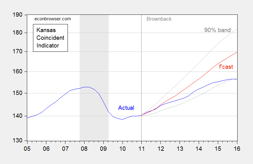
Figure 1: Coincident index for Kansas (blue), ECM forecast (red), and 90% confidence band (gray). For forecast, see text. Source: Philadelphia Fed (May releases) and author’s calculations.

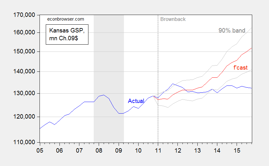
Figure 2: Kansas GDP, in millions Ch.2009$ SAAR (blue), ex post historical simulation (red), 90% prediction interval (gray lines). Forecast uses equation (1). NBER defined recession dates shaded gray. Log scale for vertical axis. Source: BEA, NBER, and author’s calculations.

In other words, even if one uses the GDP measure Ironman prefers, Kansas is still underperforming against a counterfactual. Indeed, the gap between the US and Kansas is larger using the GDP measure: 15.1% using GDP vs. 8.1% using coincident indices. So his criticism of the use of coincident indices is merely a means to distract the unwary reader.

Conclusion

Using either state GDP or coincident indices, Kansas is doing poorly against her neighbors, and against a counterfactual based on historical correlations.

Do not look for reasonable economic analysis from people who keep on asserting the same things after being shown the irrelevance of their criticisms, rely on nominal figures, infer an imminent massive GDP revision based on a misunderstanding of the nature of Chain weighted indices , and (in his MyGovCost incarnation) spin tales of a conspiracy asserting the US Government’s active destabilization of the world economy in order to lower borrowing costs.

Postscript: Ironman asserts that real Kansas GDP stripped of agriculture and manufacturing looks much better. Unfortunately, his graph in his post plots a series where he calculated Kansas GDP ex-agriculture and manufacturing by simply subtracting real agriculture and real manufacturing — both measured in Chain weighted dollars — from real GDP measured in Chain weighted dollars (the red line in Figure 3 below). This is, quite plainly, the wrong procedure, as I explained in this post.

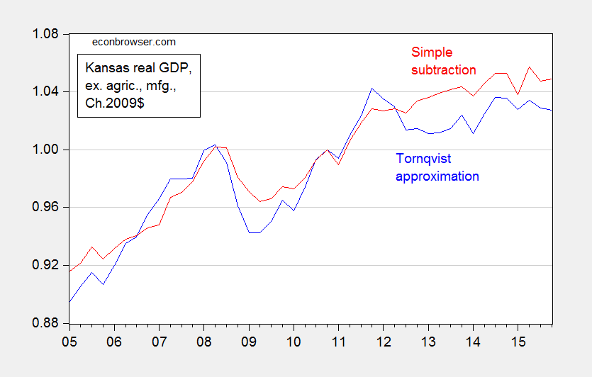
Figure 3: Kansas real GDP ex. agriculture and manufacturing, calculated using Törnqvist approximation (blue), and calculated using simple subtraction (red). Source: BEA and author’s calculations.

So a third conclusion: Don’t trust analyses from people who don’t understand the data they are working with.