Conor Jordan's Blog, page 4

Indexing in Microsoft Word

An index can be inserted at the end of a document to show the pages where certain words or phrases appear in the text. This is often used in books. When a reader wants to find out where in a document a certain topic is contained, they can check the index for information.

1. Create a new document and type the following:

Ways to fit in Activity into the Day

Low energy, tiredness, lack of enthusiasm, time constraints and wavering interest are all common barriers to taking part in regular physical activity. With many people’s lives overrun with errands, chores, tasks mounting to the ceiling, fitting in time for exercise let alone having the energy to start can seem almost impossible. For many, exercise can be seen as boring. Another mundane activity about as exciting as watching grass grow. The thought of doing any type of exercise beyond stretching to reach the remote can seem like work. However, there are many simple and effective ways to squeeze in some physical activity into your daily routine without having to lift weights in the gym or pound the treadmill for hours on end. You don’t have to be super fit to be healthy.

2. Highlight the word “physical” in the paragraph

3. In the Index group, click on Mark Entry

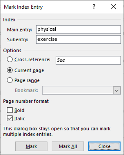
4. Type in “exercise” for Subentry

5. Check the Italic checkbox

6. Click on Mark All

7. In the Index group select Insert Index

8. Highlight the word “activity”

9. Click on Mark Entry in the Index group

10. Under Options click on Cross-reference

11. After See type in “exercise”

12. Click on the Mark button

13. Insert a Page Break at the end of the document

14. Type “Index”

15. In the Index group, select Insert Index

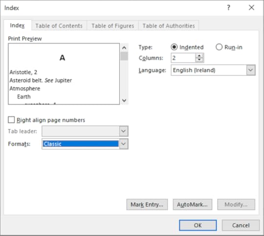
16. In Formats choose Classic

17. Click OK

18. An index at the end of the document has been created

19. Change the word 'activity' to 'exertion' in the document

20. Right-click on the index and select Update Field to update an index or press the F9 key

21. The index has been updated

22. Save the document as “Index”

To learn more about advanced Microsoft Word features, click on the book cover below:

Linking Tables in a Database

Creating Relationships

Microsoft Access allows you to link tables together so that records are maintained. For example, a primary table containing information about Customers such as Name, Address and Telephone number may be linked to Products Ordered. This will establish a link between customer details and the products they have ordered.

1. Create a table called ‘Customer Details’ with the following field names:

2. Customer Ref, First Name, Surname, Address, Telephone No.

3. Fill in details for each customer, for example:

Customer Ref: 01265 First Name: James Surname: Smith Address: 35 Main Street Telephone No. : 017384673

4. Create another table called Orders with the following field names:

Order Ref, Customer Ref, Order Date & Order Cost

5. Fill in the details for each order making sure some customers order more than one product and the Customer Ref field matches the entries in the Customer Details table:

Order Ref: 46536 Customer Ref: 01265 Order Date: 05/6/2020 Order Cost: €24.99

6. Save the database and leave it open

One-to-Many Relationships

A one-to-many relationship is when a primary table containing one field of data is linked to a table with all the details for that field. For example, a table containing Contact Details can be held in one table and can be related to a Company table where all the details for that company are held only once. This is a useful way of storing information about customers, products and companies.

1. On the Database Tools tab in the Relationships group, click on Relationships

2. In the Show Table dialog box, select the Customer Details table and click on Add

3. Do the same for the Orders table

4. Click and drag the Customer Ref field in the Customer Details table to the Customer Ref field in the Orderstable

5. In the Edit Relationships dialog box, click on the Create button

6. A One-To-Many relationship type is created

7. Return to the Customer Details table

8. Click on the Expand symbol to reveal the order details related to James Smith

9. This is called a Subdatasheet

10. Save the database

Enforcing Referential Integrity

This prevents Primary Key data in the main table from being changed or deleted or any data being changed or deleted in the Primary Table. In this example, Enforcing Referential Integrity will prevent details in the Customer Details table from being deleted or changed and data in the Customer Ref field for both tables from being changed or deleted. This is a useful feature that prevents accidental deletion or alteration of information within a database.

1. Right-click on the relationship between both tables

2. Choose Edit Relationship

3. Click on the Enforce Referential Integrity checkbox

4. Click OK

5. Save the database and close it.

To learn more about Microsoft Access, check out the Advanced ICDL Databases book below:

Database Functions in Excel

Database functions are used to perform calculations based on specified criteria. For instance, the Dsum function can be used to add cells that are above a certain value. Database functions are used when the user only wants to perform calculations on specific cells.

Dsum

This function adds numbers within a database depending on specified criteria. A database in a worksheet is a range of cells that contain numerical information.

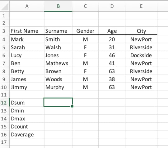
1. Create the following table in a blank worksheet:

2. On the Formula tab in the Function Library select Insert Function

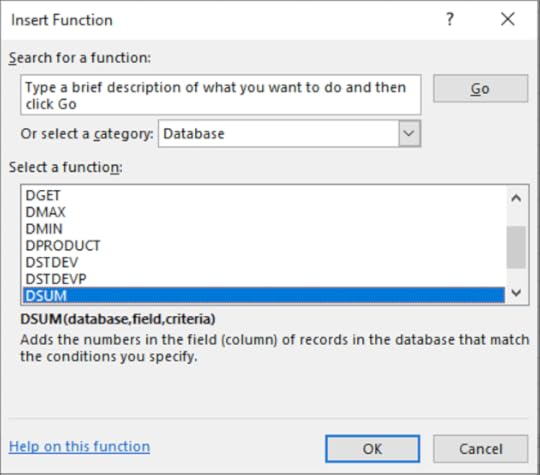
3. Select the Database category

4. Choose Dsum

5. Click OK

6. Save the workbook and keep it open

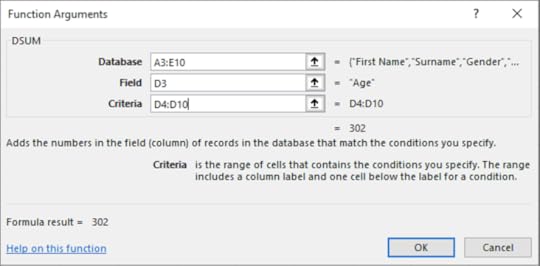
7. Select A3:E10 for the Database textbox

8. In the Field textbox type in D3

9. In the Criteria textbox, select D4:D10

10. Click OK

This function finds the minimum value out of a selected range of cells depending on specified criteria. This is useful as it can find the lowest value from a large selection of cells in a database.

1. On the Formula tab in the Function Library select Insert Function

2. Select the Database category

3. Choose Dmin

4. Click OK

5. Enter the following information into each textbox:

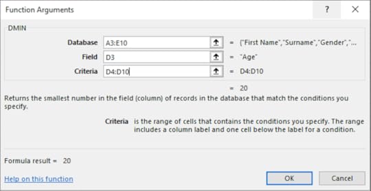
Click OK

This function finds the maximum value out of a range of selected cells in a database. This will be calculated depending on criteria specified in the function e.g. find the maximum value in a range based on certain values.

1. On the Formula tab in the Function Library select Insert Function

2. Select the Database category

3. Choose Dmax

4. Click OK

5. Enter the following information into each textbox:

6. Click OK

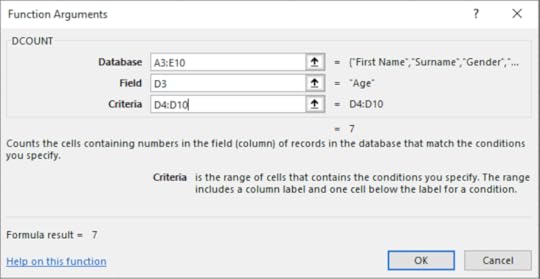
Dcount

This function counts the number of cells depending on certain criteria. For instance, if you want to find the range of cells that are below a certain number, this function will count all the cells that are below this specified number.

1. On the Formula tab in the Function Library select Insert Function

2. Select the Database category

3. Choose Dcount

4. Click OK

5. Enter the following information into each textbox:

6. Click OK

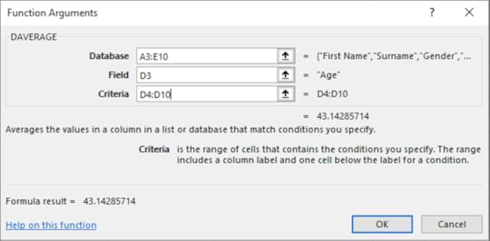
This function averages the values in a column in a database that meet specified conditions, e.g. average all of the numbers that are above 30 in a list.

1. On the Formula tab in the Function Library select Insert Function

2. Select the Database category

3. Choose Daverage

4. Click OK

5. Enter the following information into each textbox:

6. Click OK

To learn more about Advanced Excel features, click on the book cover below:

Custom Number Formats in Excel

Users of spreadsheets can determine how numbers will appear according to different formats. Custom number formats allow users to adjust how dates and time appears, whether a digit should appear in a range of cells or whether there should be a thousand or decimal separator. This is useful as it keeps the same formatting for a range of cells in a spreadsheet.

d Day number e.g. 4

m Month e.g. 6

h hours

# Displays only digits

0 Displays leading zeros

? Adds spaces either side of decimal point

, Thousands separator

. Decimal separator

Custom Number Formats

1. Open a new workbook

2. Enter 25000 into cell A2

3. On the Home tab, click Format, select Format Cells

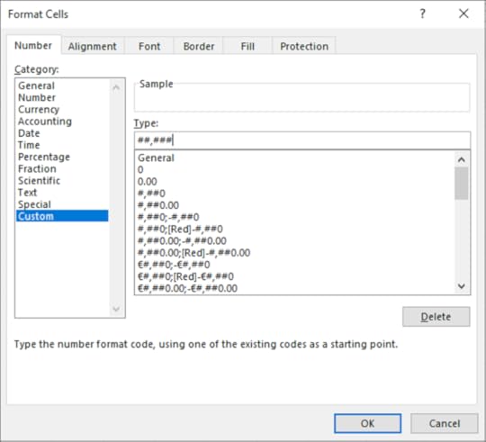
4. Within the Number tab click Custom

5. In the Type box enter ##,###

6. Click OK

7. The format of the cells will change

8. In cell B2 press Ctrl+; (Semi-Colon) to enter today’s date.

9. Display the Format Cells dialog box and click the Custom category

10. Enter ddd dd mmmm yy in the Type box to create Tue 14 April 2020

Learn more about Excel by clicking the image below or visit www.digidiscover.com/books

Captions in Microsoft Word

A caption is text that accompanies a picture. The position, formatting and type of caption can be determined by applying a range of settings. Users can choose what text appears above or below a picture. This is a useful way of labelling an image in a document.

1. Open a blank document

2. Insert an online picture of your choice into the document

3. On the References tab in the Captions group, click on Insert Captions

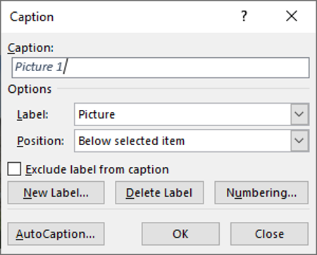
4. Click on the New Label button

5. Type in a suitable caption to accompany the picture and click OK

6. Click OK again

7. A caption has been created

8. Save the document as ‘Caption’

Deleting Captions

1. Open the Caption dialog box again

2. Click on Delete Label

3. Click OK

4. The label is deleted

Captions can also be applied to tables. The format, position and type of caption can be chosen to suit the user’s preferences. Users can choose where the caption appears and the text within the caption.

1. Create a new document

2. Insert a table with 3 columns and 4 rows

3. On the References tab in the Captions group, click on Insert Captions

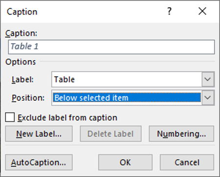
4. Change the Position to Below Selected Item

5. Click OK

Caption Numbering

1. Open the Caption dialog box again

2. Click on Numbering

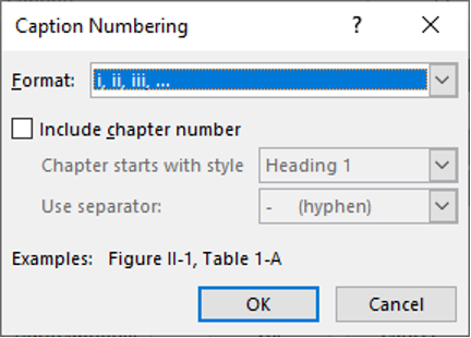
3. Change the Format to i, ii, iii, …

4. Click OK

5. Click OK again

6. Numbering has been applied to the caption

7. Save the document as ‘Table Captions’

To learn more advanced word processing features visit www.digidiscover.com/books

Charts & Sparklines in Excel

Combined Chart

You can display and compare two sets of data using a combined line and bar chart or line and area chart. This type of chart gets its information from two sources and displays them together. Often the chart contains different colours for each source so comparing and contrasting the data is made easier.

1. Create the following table:

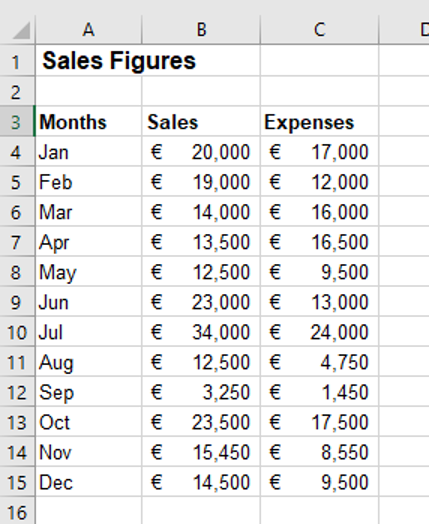
2. Highlight cells A3:C15

3. On the Insert tab in the Charts group, click on Combo Chart

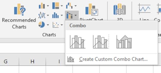
4. Select Clustered Column – Line

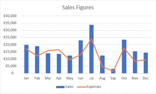
5. Change the Chart Title to “Sales Figures”

6. Save the workbook as “Combo Chart”

Sparklines

Sparklines are mini charts placed in single cells representing data from a single row. This can be useful to show information in chart form in a single cell.

1. With the “Combo Chart” still open, highlight the range of cells A4:C4

2. On the Insert tab in the Sparklines group, select Line

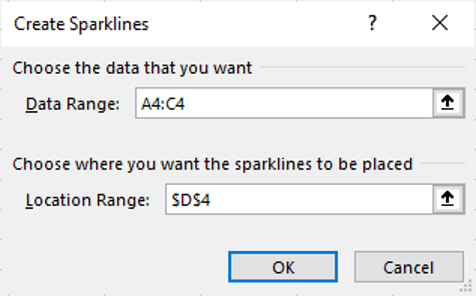
3. In the Location Range text box, select cell D4

4. Click OK

Changing a Sparkline

1. On the Sparkline Tools – Design tab in the Type group, select Column

2. Use the Fill Handle to copy the Sparklines from D4:D15

Delete a Sparkline

1. With cells D4:D15 selected, on the Sparkline Tools – Design tab in the, select Clear

Learn more about Excel features at www.digidiscover.com/books

Linking & Embedding in Microsoft Word

Linking & Embedding

Links can be placed in a document tying them to other documents or files. When you make a change in a document, this is reflected in the linked document. Embedding an object means placing an object in a document without a link. When you make a change in the document, there is no change reflected in the other document. This is a useful feature that allows you to have the option of creating links that update information in a document or keep documents separate.

Open a new document On the Insert tab in the Illustrations group click on the Chart button and choose a Pie Chart On the Insert tab in the Text group, click on the Object button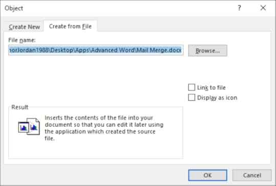

4. Select the Create From File tab and click on the Browse button

5. Navigate to your documents folder and select the document you wish to make a link to

6. Select the Link to File checkbox and click OK

7. The linked text will appear in the document beneath the pie chart

8. Save the document as “Linked”

9. Open the original document and make a change

10. Save the document

11. Re-open the “Linked” document

12. Select Yes in the dialog box

13. The changes will be updated in the linked document

14. Save the document

Display as Icon

Open the “Linked” document On the Insert tab in the Text group, click on the Object button Select the Display as Icon checkbox Click OK The object will be displayed as an icon in the document Save the document as ‘Display as Icon’ Leave the document open

Break a Link

Users can break a link between files when there is no longer a need for a link. This means that changes to an original file will not be reflected in the document.

Open the ‘Display as Icon’ document On the File tab select Info On the bottom right-hand corner of the screen click on Edit Links to Files Select the Source File and click on Break Link Click on Yes The link is now broken between both documents Save the document as ‘Broken Link’

Embedding Data

When a user wants to place an object in a document, they can embed it without creating a link. This means that the object that is placed in the document can only be changed in that document.

Open a new document On the Insert tab in the Text group click on Object Select the Create from File tab and click on Browse Navigate to the exercises folder and select ‘Pie Chart’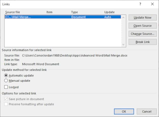

5. Do not select the Link to File checkbox

6. Click OK

7. You can now make changes to the chart by double-clicking on it and editing the data

8. Select the chart and press Delete to remove the object

9. Close the document without saving

For more information about Advanced Word Processing, click on the image below:

Input Masks in Microsoft Access

Input masks define how data is entered and shown in a field. Symbols are used to define what information should be entered, and how it will be displayed. For example, if you have a field in a database that requires six letters to be entered, the input mask would be LLLLLL. Input masks help keep data entry consistent within a database and reduce the chance of errors occurring.

Examples of Input Masks:

L = Letter (Required Entry)

? = Letter (Entry Not Required)

A = Letter or Number (Required Entry)

A = Letter or Number (Entry Not Required)

& = Any Character or Space (Required Entry)

C = Any Character or Space (Entry Not Required)

0 = Number (Required Entry)

9 = Number (Entry Not Required)

# = Number, Space, + or –

., = Decimal Point and thousands separators

:/ = Date and time separators

< = Converts characters to the right to lowercase

> = Converts characters to the right to uppercase

\ = Makes the character that follows to be displayed as itself e.g. \H will be displayed as H

Create a table containing contact details with fields named Name, Address and Telephone. Enter relevant details into the table Open the table in Design View Select the Telephone field Click in the Input Mask field property Enter (00) 0000000 for the Input Mask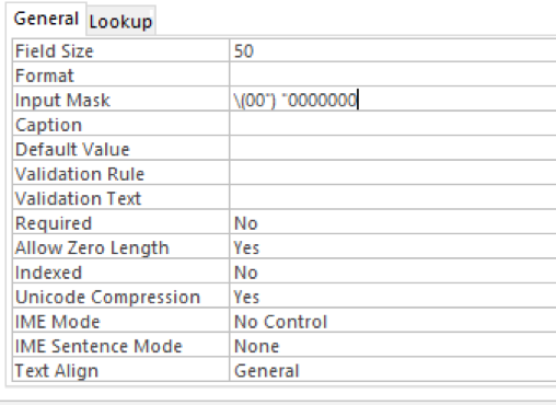

6. Return to Datasheet View and try and enter a new telephone number for the last record

7. The table will only accept telephone numbers in the correct format

8. Display the Design View

9. To the right of the Input Mask property, click on the dots. This will display the Input Mask Wizard

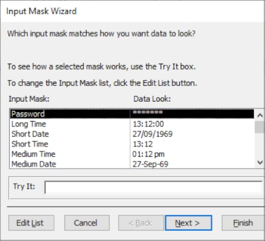
10. Scroll down through the list of Input Masks available until you reach the Telephone number Input Mask

11. Click on Next

12. Click Finish

13. When you return to Datasheet View, the new Input Mask will be applied to the Telephone field

14. Save the database

For further database tips and tricks, click on the book below:

Statistical Functions

Statistical Functions

Statistical functions perform calculations based on certain criteria. Countif is used to count a range of selected cells that meet a specified criteria. Countblank counts the number of blank cells in a range of cells. Rank.Eq displays the rank of a selected cell within a range of cells. These are useful functions to perform calculations on data contained within a worksheet.

Countif

1. Create the following table:

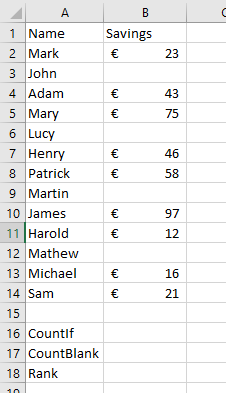
2. Select cell B16

3. On the Formulas tab in the Function Library, select More Functions then Statistical

4. Select CountIf

5. Select the Range B2:B14

6. Enter the Criteria as >30

7. Click OK

8. This will Count the cells with a value greater than 30

Countblank

Select cell B17 On the Formulas tab in the Function Library, select More Functions then Statistical Select CountBlank Select the cell Range B2:B14 Click OK This Counts the Blank cells in the Range

Rank.Eq

Select cell B18 On the Formulas tab in the Function Library, select More Functions then Statistical Select Rank.Eq In the Number text box select cell B13 In the Ref text box select the range B2:B14 Click OK This will find the rank of the selected number in that range Save the spreadsheet as “Statistical Functions”

For more information about Advanced Spreadsheet features, click on the paperback cover below:

Creating an Organisation Chart in PowerPoint

Organisation Chart

This is an overview of who is in a company or department. Each employee has a place on the chart depending on where they rank in the company or department. It is useful for displaying the structure of a group or company. The organisation chart can be formatted to suit the users needs.

1. Create a blank presentation

2. Insert a new slide using the Title and Content layout

3. Click on Insert a SmartArt Graphic

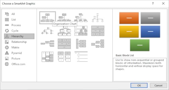
4. On the left of the dialog box, choose Hierarchy

5. Select Organisation Chart

6. Click OK

7. Click in the Text box to enter text into the organisation chart

8. Hold Shift and press Enter to type beneath the name of the person in the text box

9. Click on the text box below the Director

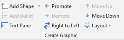
10. On the SmartArt Tools Design tab in the Create Graphic group, click on Add Shape

11. A new shape has been added to the Organisation Chart

12. Click and drag on the handles around the Organisation Chart to resize it

13. Click on the chart border and move the mouse to move the chart around

14. Click on a Text Box and press the Delete key to remove it

15. On the second row of the chart, click on the Text Box on the right

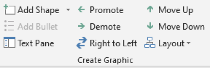
16. In the Create Graphic group, click on Promote

17. Click on a Text Box on the bottom of the chart

18. On the Home tab in the Clipboard group, select Cut

19. Select the top row of the Organisation Chart

20. On the Home tab in the Clipboard group, select Paste

21. With that Text Box still selected, in the Create Graphic group, click on Demote to move the text box down

22. Save the presentation as ‘Organisation Chart’

For more Advanced PowerPoint tutorials, click on the book image below: