Conor Jordan's Blog, page 2

How to Use Calculations in Forms with Microsoft Access

A Text Box form control creates an unbound control that is unlinked to any data source with a Label and Text Box. This can be used to perform calculations and labelling the resulting calculation.

Bound form controls obtains data from a source or a field. Unbound form controls are not linked to a data source and are calculated. Unbound form controls are calculated using other information from the database.

Calculations can use any of the mathematical symbols (+, -, *, /) and expressions such as Average, Sum, Max and Min.

1. Download the work files associated with Advanced Database at www.digidiscover.com/downloads

2. Open the Computer Store database

3. Open the Products Report report

4. Switch to Design View and enlarge the Detail area

5. Click on the Text Box button on the Design tab in the Controls group

6. Create an unbound control beneath Items Sold

7. In the Tools group, select Property Sheet to display the control’s properties

8. Click on the Data tab on the Property Sheet pane and select Control Source. Choose Product as the Control Source

9. Enter the following expression into the textbox:

=[Price]*[Items Sold]

10. Name the label Product Total

11. Resize the label and text box so it aligns with the other text boxes

12. Click inside the text box and on the Property Sheet pane select the Format tab

13. Change the format to Euro

14. Switch to Form View to see the result

15. Return to Design View. Add another text box beneath the Product Total

16. Enter in the following expression:

=IIf([Product_Total]>1000,“High Value”,“Low Value”)

17. This expression will show the text “High Value” if the product total is above €1,000 and display “Low Value” if the product total is lower than €1,000

18. Enter a label of Product Value

19. Save the form and close it

To learn more about advanced database features check out the Advanced ICDL Databases paperback:

Database Functions in Excel

Database functions are formulas used in spreadsheets to calculate amounts based on tables of information that meet certain criteria. For example, this type of formula may be used to calculate the total salary above €20,000 of employees in a table. The DSUM function adds numbers in a table of data based on specified criteria. The DMAX, DMIN, DCOUNT & DAVERAGE functions are also used to calculate amounts in a table based on specified criteria.

Dsum

This function adds numbers within a database depending on specified criteria. A database in a worksheet is a range of cells that contain numerical information.

1. Download the Advanced ICDL Spreadsheets work files folder from www.digidiscover.com/downloads

2. Open the Database Function workbook

3. On the Formula tab in the Function Library select Insert Function

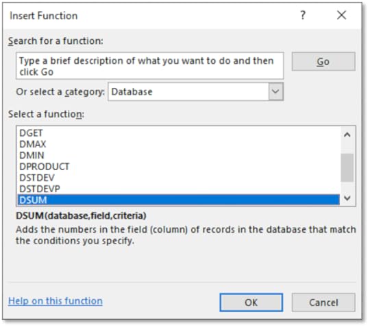
4. Select the Database category

5. Choose Dsum

6. Click OK

7. Save the workbook and keep it open

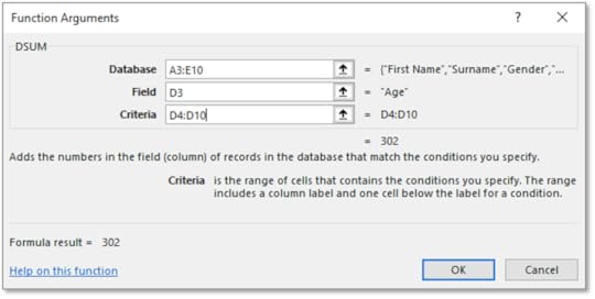
8. Select A3:E10 for the Database textbox

9. In the Field textbox type in D3

10. In the Criteria textbox, select D4:D10

11. Click OK

12. Save the workbook and leave it open

Dmin

This function finds the minimum value out of a selected range of cells depending on specified criteria. This is useful as it can find the lowest value from a large selection of cells in a range of data in a table.

1. With the Database Function workbook open, on the Formula tab in the Function Library select Insert Function

2. Select the Database category

3. Choose Dmin

4. Click OK

5. Enter the following information into each textbox:

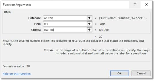
6. Click OK

7. Leave the workbook open

Dmax

This function finds the maximum value out of a range of selected cells in a database. This will be calculated depending on criteria specified in the function e.g. find the maximum value in a range based on certain values.

1. Open the Database Function workbook

2. On the Formula tab in the Function Library select Insert Function

3. Select the Database category

4. Choose Dmax

5. Click OK

6. Enter the following information into each textbox:

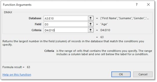
7. Click OK

8. Save the workbook

Dcount

This function counts the number of cells depending on certain criteria. For instance, if you want to find the range of cells that are below a certain number, this function will count all of the cells that are below this specified number.

1. Open the Database Function workbook

2. On the Formula tab in the Function Library select Insert Function

3. Select the Database category

4. Choose Dcount

5. Click OK

6. Enter the following information into each textbox:

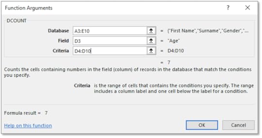
7. Click OK

8. Save the workbook

Daverage

This function averages the values in a column in a list of database that meet specified conditions, e.g. average all of the numbers that are above 30 in a list.

1. Open the Database Function workbook

2. On the Formula tab in the Function Library select Insert Function

3. Select the Database category

4. Choose Daverage

5. Click OK

6. Enter the following information into each textbox:

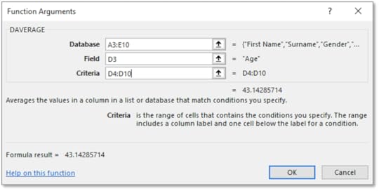
7. Click OK

8. Save the workbook and close it

To learn more about advanced spreadsheet features check out the Advanced ICDL Spreadsheets paperback available on Amazon:

Custom Number Formats in Excel

Users of spreadsheets can determine how numbers will appear according to different formats. Custom number formats allow users to adjust how dates and time appears, whether a digit should appear in a range of cells or whether there should be a thousand or decimal separator. This is useful as if keeps the same formatting for a range of cells in a spreadsheet.

d Day number e.g. 4

m Month e.g. 6

h hours

# Displays only digits

0 Displays leading zeros

? Adds spaces either side of decimal point

, Thousands separator

. Decimal separator

Custom Number Formats

1. Open the “Sales” workbook

2. On the Home tab, click Format, select Format Cells

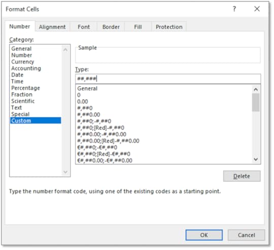
3. Within the Number tab click Custom

4. In the Type box enter ##,###

5. Click OK

6. The format of the cells will change

7. In cell B2 press Ctrl+; (Semi-Colon) to enter today’s date.

8. Display the Format Cells dialog box and click the Custom category

9. Enter ddd dd mmmm yy in the Type box to create Tue 14 April 2020

To learn more about advanced spreadsheet features click on the paperback cover below:

Data Tables in Excel

A data table is used to see how altering one variable in a formula affects the result of that formula e.g. calculating the amount of interest on a savings account at different interest rates. The monthly repayment amount stays the same but is calculated at different interest rates. Rather than typing in several formulas for each interest rate, a data table can be used to quickly calculate information. This is a more efficient way of calculating variable amounts using formulas.

1. Open the “Repayments on Loan” workbook 2. Highlight cells A9:A19 3. On the Home tab select Series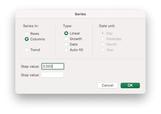 4. For Series In select Columns 5. For Step Value enter 0.005 6. Click OK 7. This will create a variable interest rate that increases by 0.5% for each calculation 8. In cell B9 type in =B6 9. Highlight cells A8:B19 10. On the Data tab select What-If Analysis and choose Data Table 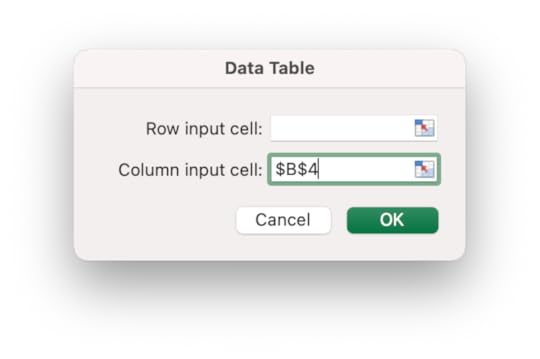11. Highlight cell D4 for the Column Input Cell 12. This uses the standard interest rate on the loan to calculate the variable interest rate in the data table 13. Click OK 14. Change the cell range B9:B19 to currency with two decimal places 15. The Data Table will calculate the amount monthly repayments will be based on variable interest rates 16. ave the workbook as “Loan”

Two Input Data Table

A two-input data table is used to see how changing two variables in a formula affects the result of that formula e.g. calculating the amount of interest on a savings account at variable interest rates at different periods of time. The interest rate variable changes and the length of the savings period also changes. This produces a different amount depending on changing interest rates and different periods of time. A two-input data table uses two changing variables compared with one changing variable in a one input data table.

1. Open the workbook “Loan” 2. Delete the contents of cells in the range B9:B18 3. Cut and paste the range B8:G8 to A8:F8 4. The numbers across the top represent the term of the loan in months 5. Highlight cells A8:F19 6. On the Data tab click on What-If Analysis and choose Data Table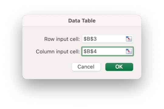

7

7. Select cell B3 for the Row Input Cell 8. This includes the standard term of the loan to be included in the data table containing a variable loan term 9. Select cell B4 for the Column Input Cell 10. This included the standard interest rate of the loan to be included in the data table containing a variable loan term 11. Click OK 12. Apply a currency format to the cell range B9:F19 13. A Data Table will be created displaying the monthly repayment amount depending on the variable interest rate and the variable term of the loan 14. Save the workbook and close it

To learn more advanced Excel features, click on the book cover image below:

Database Concepts with Microsoft Access

Types of Database Models

Databases are used to store and access data in many ways. They are often used for websites e.g. containing price and product information on an e-commerce site. Website content management systems allow users to make changes to web content without having to have technical knowledge. Databases can be used for business involved in distribution, logistics, shipping and inventories. They can be used to store data about customers such as contact details and home address. This information can then be modified and updated.

Hierarchal databases are similar to a tree structure. Records are stored in groups of master/subordinate relationships. There may be a high priority table e.g. containing customer details and relationships between many product tables which would be subordinate. This model is fast and simple to use but only contains one-to-many relationships.

Relational databases have data organised in a series of related tables. It can be manipulated in many different ways. This type of database is easy to create, access and add to. These types of databases may be used in companies where employee details for different departments are stored and are related to each other.

Object-orientated databases have data represented by objects. Not all of these models support Structured Query Language. SQL is a language used in Microsoft Access when it runs Queries. Website content management systems often use this type of database e.g. in a shop at the cashier.

Stages of a Database

Stage 1 – Design

The design must be clear and consider what the database will be used for. Future use should also be taken into account when designing a database. How will it output data? What will the result of the database be? How will it be used to serve the needs of the people who access it?

Stage 2 – Creation

This involves developing tables, data input, relationships, forms, queries and reports. This process needs to be followed carefully to ensure that there is a clear understanding of the links between tables and the output of selected databases.

Stage 3 – Data Entry

This stage involves entering information into a database. This is a long, labour intensive process and requires a skilled user. There are many features in Microsoft Access that can limit the chance of errors occurring such as data validation methods that only allow certain information to be entered and input masks where data entered must be of a certain format.

Stage 4 – Data Maintenance

This involves adding new information and removing unnecessary data from a database to make it more efficient. This process is carried out on a continual basis as information changes e.g. contact details of customers or product updates.

Stage 5 – Information Retrieval

Information is retrieved and organised using queries, forms and reports. Users may only be allowed to use sections of a database because of restrictions.

Applications of Databases

Databases can be used for dynamic websites where data is retrieved and updated for information such as product details or prices. Databases are often used to manage mailing lists where email details are stored. These databases can then be updated when contact details change.

For instance, when a customer entering contact details including name, address, email and date of birth into a shopping website, this data is retrieved automatically and updated using company databases. This information can then be related to products purchased by that customer and a record of this information will then be stored in the organisation’s databases.

Website content management systems use databases where users without technical skills can edit information e.g. product sales details. The user may input data without having to know coding languages. This makes data entry more effective and efficient.

Customer Relationship Management Systems uses databases to store and retrieve customer details in an organisation. Information such as name and address can be used by a company. This information can then be updated whenever customers’ details change.

This type of system may be used in a hotel, for instance where an established content management system is used by a staff member. The contact details of the guest is stored in a client database, information about the amount charged, length of stay and room stayed in may also be included in separate databases. This information can then be changed and updated as different guests arrive and leave the hotel.

To learn more about Databases with Microsoft Access, click on the book cover image below:

Automation in Microsoft Word

AutoFormat formats an entire document using a pre-set style. This is useful if you want to apply a consistent style to the document. It is an efficient way of applying a similar style to a document.

1. Open a document containing text

2. Click on the Customize Quick Access Toolbar arrow and choose More Commands

3. Under Choose Commands From select All Commands

4. Scroll down until you find AutoFormat

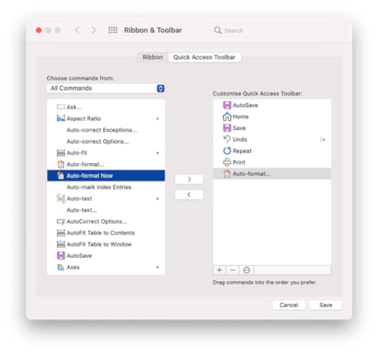
5. Click on the Right Arrow button and click Save

6. Click on the AutoFormat button

7. Select AutoFormat Now

8. Click OK

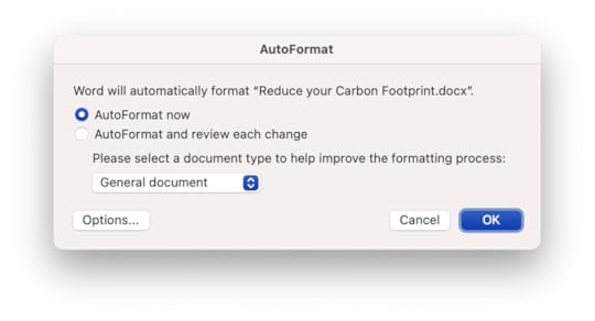
9. The document will be formatted according to the styles available

10. Save the document as "Formatted”

11. Leave the document open

AutoCorrect allows you to input words to replace other selected words. For instance, if you want your initials to display your name automatically, these settings can be applied to your document. When you type in your initials, your name will appear. It is a useful feature if you enter long, complicated words into a document frequently and want to use an abbreviation that displays the full word.

For example, if you enter hard to spell words into documents regularly, AutoCorrect can be used to efficiently enter in these details into your document.

1. Open Preferences and select AutoCorrect

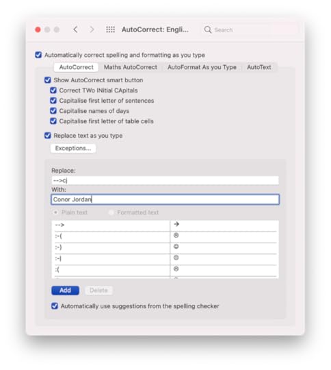
2. With the AutoCorrect tab selected, type in your initials into the Replace text box and in the With text box, type your name

3. Click OK

4. Place your cursor at the end of the document and type in your initials

5. Your full name will appear

6. Open the AutoCorrect dialog box again and locate the entry you created

7. Click on the Delete button

8. This deletes the AutoCorrect entry

9. Click OK

10. Save the document as "Autocorrect”

AutoText for text that is used frequently such as addresses or names. This is useful when repeating tasks often e.g. when creating letters. The AutoText entry can be prepared by entering in its name, category, and description.

1. Open the “Autocorrect” document & enter your name and address at the top of the document

2. Highlight the name and address at the top of the document

3. Open Preferences and select AutoText

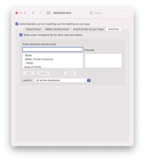
4. Click Add

5. This address will be available for use in other documents

6. Open a new document and begin typing the start of the address

7. Press Enter

8. The address will appear automatically

9. Save the document as "Auto text”

The contents of AutoText entries can be modified so that different text appears when specific initials, acronyms or abbreviations are input into a document. For example, when entering tm into a document, this can be modified from Trade Mark to trademark. AutoText entries can be deleted when they are no longer required.

1. Open the "Auto text” document

2. Open Preferences and select AutoText

3. Locate the address and type in Henry Smith for the name of the address

4. Click on the Add button

5. The address has been changed

6. Open a new document

7. Begin typing Henry Smith

8. The address will appear

9. Save the document

Delete an AutoText Entry

1. Open Preferences and select AutoText

2. Locate the address and click on Delete

3. The AutoText entry has now been deleted, save the document and close it

To learn more about advanced Word processing features, click on the book cover image below:

Days until Christmas Excel Formula

The DAYS formula in Excel will calculate the number of days between a start date and end date in a worksheet. This is a useful formula to apply to a large worksheet that contains extensive information such as employee’s workdays. It is also useful when counting down the days until Christmas!

1. Open a blank workbook

2. In cell A1, enter the title “Today”

3. In cell B1, enter the title “Days until Christmas”

4. In cell C1, enter the title “Christmas Day”

5. In cell A2, enter in the following formula:

=today()

6. This will calculate today’s date

7. In cell C2, enter in the date of Christmas (I haven’t found a formula for that yet!)

8. Highlight cell B2

9. On the Formulas tab, select Date & Time and choose the Days formula

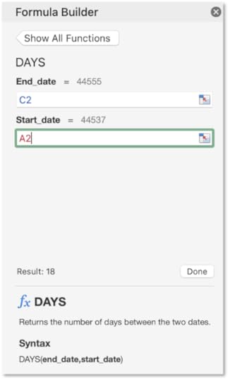
10. On the Formula Builder pane, select cell C2 for End_date

11. Select cell A2 for Start_date

12. Click on Done

13. This will calculate the number of days until Christmas!

14. Save the workbook as “Christmas Countdown” and close it

For further information about Excel formulas, click on the book cover below:

Networkdays Formula in Excel

This formula is used to calculate the total number of days worked by employees based on the start date and end date of employment. This calculation also includes holidays which are deducted from the total number of days worked. For example, when a manager is calculating annual salaries for employees, the Networkdays formula is used to work out the total amount of work days completed.

1. Open the “Employee Records” spreadsheet

2. Select cell G3

3. On the Formulas tab click on Date & Time and select the Networkdays formula

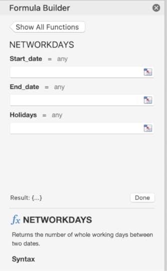
4. Select cell D3 for the Start_date input

5. Select cell E3 for the End_date input

6. Select cell F3 for the Holidays input

7. Click on the Done button

8. The total number of days worked for each employee has been calculated

9. Save the workbook and close it

For further information about advanced Excel features, click on the book cover below:

XNPV - Excel Financial Function

XNPV - Excel Financial Function

This financial function calculates the Net Present Value of a series of cashflow payments based on a set discount rate. For example, if you want to find the worth of a loan that has a fixed discount rate based on a series of payments made, the XNPV function can calculate the present value of the loan. The dates of payments made, the amount of each payment and the discount rate are included in the calculation.

1. Download the "Enterprise Loan" provided on the left

2. Notice the Discount Rate that is set to 5%

3. The payment dates are displayed alongside the payment amounts on each date

4. Select cell B21. This will be the answer cell where you calculate the Net Present Value based on the information provided

5. On the Formulas tab select Financial and select the formula XNPV

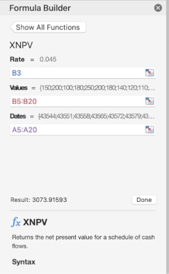
6. For the Rate text box, select B3

7. For the Values text box, select the cell range B5:B20

8. For the Dates text box, select the cell range A5:A20

9. Click on Done

10. The answer will display the Net Present Value of the loan based on the Discount Rate, Payments Made and Dates of Payments

11. Save the workbook and close it

NPV - Excel Financial Function

XNPV - Excel Financial Function

This financial function calculates the Net Present Value of a series of cashflow payments based on a set discount rate. For example, if you want to find the worth of a loan that has a fixed discount rate based on a series of payments made, the XNPV function can calculate the present value of the loan. The dates of payments made, the amount of each payment and the discount rate are included in the calculation.

1. Download the "Enterprise Loan" provided on the left

2. Notice the Discount Rate that is set to 5%

3. The payment dates are displayed alongside the payment amounts on each date

4. Select cell B21. This will be the answer cell where you calculate the Net Present Value based on the information provided

5. On the Formulas tab select Financial and select the formula XNPV

6. For the Rate text box, select B3

7. For the Values text box, select the cell range B5:B20

8. For the Dates text box, select the cell range A5:A20

9. Click on Done

10. The answer will display the Net Present Value of the loan based on the Discount Rate, Payments Made and Dates of Payments

11. Save the workbook and close it