Allen B. Downey's Blog: Probably Overthinking It, page 13

Maxima, Minima, and Mixtures

I am hard at work on the second edition of Think Bayes, currently working on Chapter 6, which is about computing distributions of minima, maxima and mixtures of other distributions.

Of all the changes in the second edition, I am particularly proud of the exercises. I present three new exercises from Chapter 6 below. If you want to work on them, you can use this notebook, which contains the material you will need from the chapter and some code to get you started.

Exercise 1

Henri Poincaré was a French mathematician who taught at the Sorbonne around 1900. The following anecdote about him is probably fabricated, but it makes an interesting probability problem.

Supposedly Poincaré suspected that his local bakery was selling loaves of bread that were lighter than the advertised weight of 1 kg, so every day for a year he bought a loaf of bread, brought it home and weighed it. At the end of the year, he plotted the distribution of his measurements and showed that it fit a normal distribution with mean 950 g and standard deviation 50 g. He brought this evidence to the bread police, who gave the baker a warning.

For the next year, Poincaré continued the practice of weighing his bread every day. At the end of the year, he found that the average weight was 1000 g, just as it should be, but again he complained to the bread police, and this time they fined the baker.

Why? Because the shape of the distribution was asymmetric. Unlike the normal distribution, it was skewed to the right, which is consistent with the hypothesis that the baker was still making 950 g loaves, but deliberately giving Poincaré the heavier ones.

To see whether this anecdote is plausible, let’s suppose that when the baker sees Poincaré coming, he hefts n loaves of bread and gives Poincaré the heaviest one. How many loaves would the baker have to heft to make the average of the maximum 1000 g?

Exercise 2

Two doctors fresh out of medical school are arguing about whose hospital delivers more babies. The first doctor says, “I’ve been at Hospital A for two weeks, and already we’ve had a day when we delivered 20 babies.”

The second doctor says, “I’ve only been at Hospital B for one week, but already there’s been a 19-baby day.”

Which hospital do you think delivers more babies on average? You can assume that the number of babies born in a day is well modeled by a Poisson distribution.

Exercise 3

Suppose I drive the same route three times and the fastest of the three attempts takes 8 minutes.

There are two traffic lights on the route. As I approach each light, there is a 40% chance that it is green; in that case, it causes no delay. And there is a 60% chance it is red; in that case it causes a delay that is uniformly distributed from 0 to 60 seconds.

What is the posterior distribution of the time it would take to drive the route with no delays?

The solution to this exercise is very similar to a method I developed for estimating the minimum time for a packet of data to travel through a path in the internet.

Again, here’s the notebook where you can work on these exercises. I will publish solutions later this week.

Think DSP v1.1

For the last week or so I have been working on an update to Think DSP. The latest version is available now from Green Tea Press. Here are some of the changes I made:

Running on Colab

All notebooks now run on Colab. Judging by my inbox, many readers find it challenging to download and run the code. Running on Colab is a lot easier.

If you want to try an example, here’s a preview of Chapter 1. And if you want to see where we’re headed, here’s a preview of Chapter 10. You can get to the rest of the notebooks from here.

No more thinkplot

For the first edition, I used a module called thinkplot that provides functions that make it easier to use Matplotlib. It also overrides some of the default options.

But since I wrote the first edition, Matplotlib has improved substantially. I found I was able to eliminate thinkplot with minimal changes. As a result, the code is simpler and the figures look better.

Still using thinkdsp

I provide a module called thinkdsp that contains classes and functions used throughout the book. I think this module is good for learners. It lets me hide details that would otherwise be distracting. It lets me present some topics “top-down”, meaning that we learn how to use some features before we know how they work.

And when you learn the API provided by thinkdsp, you are also learning about DSP. For example, thinkdsp provides classes called Signal, Wave, and Spectrum.

A Signal represents a continuous function; a Wave represents a sequence of discrete samples. So Signal provides make_wave, but Wave does not provide make_signal. When you use this API, you understand implicitly that this is a one-way operation: you can sample a Signal to get a Wave, but you cannot recover a Signal from a Wave.

On the other hand, you can convert from Wave to Spectrum and from Spectrum to Wave, which implies (correctly) that they are equivalent representations of the same information. Given one, you can compute the other.

I realize that not everyone loves it when a book uses a custom library like thinkdsp. When people don’t like Think DSP, this is the most common reason. But looking at thinkdsp with fresh eyes, I am doubling down; I still think it’s a good way to learn.

Less object-oriented

Nevertheless, I found a few opportunities to simplify the code, and in particular to make it less object-oriented. I generally like OOP, but I acknowledge that there are drawbacks. One of the biggest is that it can be hard to keep an inheritance hierarchy in your head and easy to lose track of what classes provide which methods.

I still think the template pattern is a good way to present a framework: the parent class provides the framework and child classes fill in the details.

However, based on feedback from readers, I have come to realize that object-oriented programming is not as universally known and loved as I assumed.

In several places I found that I could eliminate object-oriented features and simplify the code without losing explanatory power.

Pretty, pretty good

Coming back to this book after some time, I think it’s pretty good. If you are interested in digital signal processing, I think the computation-first approach is a good way to get started. And if you are not interested in digital signal processing, maybe I can change your mind!

Here are the links again:

Here’s the latest version from Green Tea Press. Here’s a preview of Chapter 1. that you can run in a browser.And here’s a preview of Chapter 10. You can get to the rest of the notebooks from here.

Bayesian hypothesis testing

I have mixed feelings about Bayesian hypothesis testing. On the positive side, it’s better than null-hypothesis significance testing (NHST).

And it is probably necessary as an onboarding tool: Hypothesis testing is one of the first things future Bayesians ask about; we need to have an answer.

On the negative side, Bayesian hypothesis testing is often unsatisfying because the question it answers is not the most useful question to ask.

To explain, I’ll use an example from Bite Size Bayes, which is a series of Jupyter notebooks I am writing to introduce Bayesian statistics.

In Notebook 7, I present the following problem from David MacKay’s book, Information Theory, Inference, and Learning Algorithms:

“A statistical statement appeared in The Guardian on Friday January 4, 2002:

“When spun on edge 250 times, a Belgian one-euro coin came up heads 140 times and tails 110. ‘It looks very suspicious to me’, said Barry Blight, a statistics lecturer at the London School of Economics. ‘If the coin were unbiased the chance of getting a result as extreme as that would be less than 7%’.”

“But [asks MacKay] do these data give evidence that the coin is biased rather than fair?”

I start by formulating the question as an estimation problem. That is, I assume that the coin has some probability, x, of landing heads, and I use the data to estimate it.

If we assume that the prior distribution is uniform, which means that any value between 0 and 1 is equally likely, the posterior distribution looks like this:

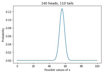Posterior distribution of x, which is the probability of heads, given a uniform prior.

This distribution represents everything we know about x given the prior and the data. And we can use it to answer whatever questions we have about the coin.

So let’s answer MacKay’s question: “Do these data give evidence that the coin is biased rather than fair?”

The question implies that we should consider two hypotheses:

The coin is fair.The coin is biased.

In classical hypothesis testing, we would define a null hypothesis, choose a test statistic, and compute a p-value. That’s what the statistician quoted in The Guardian did. His null hypothesis is that the coin is fair. The test statistic is the difference between the observed number of heads (140) and the expected number under the null hypothesis (125). The p-value he computes is 7%, which he describes as “suspicious”.

In Bayesian hypothesis testing, we choose prior probabilities that represent our degree of belief in the two hypotheses. Then we compute the likelihood of the data under each hypothesis. The details are in Bite Size Bayes Notebook 12.

In this example the answer depends on how we define the hypothesis that the coin is biased:

If you know ahead of time that the probability of heads is exactly 56%, which is the fraction of heads in the dataset, the data are evidence in favor of the biased hypothesis.If you don’t know the probability of heads, but you think any value between 0 and 1 is equally likely, the data are evidence in favor of the fair hypothesis.And if you have knowledge about biased coins that informs your beliefs about x, the data might support the fair or biased hypothesis.

In the notebook I summarize these results using Bayes factors, which quantify the strength of the evidence. If you insist on doing Bayesian hypothesis testing, reporting a Bayes factor is probably a good choice.

But in most cases I think you’ll find that the answer is not very satisfying. As in this example, the answer is often “it depends”. But even when the hypotheses are well defined, a Bayes factor is generally less useful than a posterior distribution, because it contains less information.

The posterior distribution incorporates everything we know about the coin; we can use it to compute whatever summary statistics we like and to inform decision-making processes. We’ll see examples in the next two notebooks.

Correlation, determination, and prediction error

This tweet appeared in my feed recently:

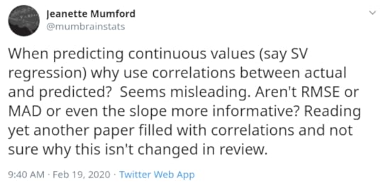
I wrote about this topic in Elements of Data Science Notebook 9, where I suggest that using Pearson’s coefficient of correlation, usually denoted ρ, to summarize the relationship between two variables is problematic because:

Correlation only quantifies the linear relationship between variables; if the relationship is non-linear, correlation tends to underestimate it.Correlation does not quantify the “strength” of the relationship in terms of slope, which is often more important in practice.

For an explanation of either of those points, see the discussion in Notebook 9. But that tweet and the responses got me thinking, and now I think there are even more reasons correlation is not a great statistic:

It is hard to interpret as a measure of predictive power.It makes the relationship between variables sound more impressive than it is.

As an example, I’ll quantify the relationship between SAT scores and IQ tests. I know this is a contentious topic; people have strong feelings about the SAT, IQ, and the consequences of using standardized tests for college admissions.

I chose this example because it is a topic people care about, and I think the analysis I present can contribute to the discussion.

But a similar analysis applies in any domain where we use a correlation to quantify the strength of a relationship between two variables.

SAT scores and IQ

According to Frey and Detterman, “Scholastic Assessment or g? The relationship between the Scholastic Assessment Test and general cognitive ability“, the correlation between SAT scores and general intelligence (g) is 0.82.

That’s just one study, and if you read the paper, you might have questions about the methodology. But for now I will take this estimate at face value. If you find another source that reports a different correlation, feel free to plug in another value and run my analysis again.

In the notebook, I generate fake datasets with the same mean and standard deviation as the SAT and the IQ, and with a correlation of 0.82.

Then I use them to compute

The coefficient of determination, R²,The mean absolute error (MAE),Root mean squared error (RMSE), andMean absolute percentage error (MAPE).

In the SAT-IQ example, the correlation is 0.82, which is a strong correlation, but I think it sounds stronger than it is.

R² is 0.66, which means we can reduce variance by 66%. But that also makes the relationship sound stronger than it is.

Using SAT scores to predict IQ, we can reduce MAE by 44%, we can reduce RMSE by 42%, and we can reduce MAPE also by 42%.

Admittedly, these are substantial reductions. If you have to guess someone’s IQ (for some reason) your guesses will be more accurate if you know their SAT scores.

But any of these reductions in error is substantially more modest than the correlation might lead you to believe.

The same pattern holds over the range of possible correlations. The following figure shows R² and the fractional improvement in RMSE as a function of correlation:

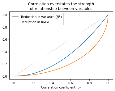
For all values except 0 and 1, R² is less than correlation and the reduction in RMSE is even less than that.

Summary

Correlation is a problematic statistic because it sounds more impressive than it is.

Coefficient of determination, R², is a little better because it has a more natural interpretation: percentage reduction in variance. But reducing variance it usually not what we care about.

A better option is to choose a measure of error that is meaningful in context, possibly MAE, RMSE, or MAPE.

Which one of these is most meaningful depends on the cost function. Does the cost of being wrong depend on the absolute error, squared error, or percentage error? If so, that should guide your choice.

One advantage of RMSE is that we don’t need the data to compute it; we only need the variance of the dependent variable and either ρ or R². So if you read a paper that reports ρ, you can compute the corresponding reduction in RMSE.

But any measure of predictive error is more meaningful than reporting correlation or R².

The details of my analysis are in this Jupyter notebook.

The Girl Named Florida

In The Drunkard’s Walk, Leonard Mlodinow presents “The Girl Named Florida Problem”:

“In a family with two children, what are the chances, if [at least] one of the children is a girl named Florida, that both children are girls?”

I added “at least” to Mlodinow’s statement of the problem to avoid a subtle ambiguity.

I wrote about this problem in . As you can see in the comments, my explanation was not met with universal acclaim.

This time, I want to take a different approach.

First, to avoid some real-world complications, let’s assume that this question takes place in an imaginary city called Statesville where:

Every family has two children.50% of children are male and 50% are female.All children are named after U.S. states, and all state names are chosen with equal probability.Genders and names within each family are chosen independently.

Second, rather than solve it mathematically, I’ll demonstrate it computationally:

You can view my solution in this Jupyter notebook,Or you can run it yourself on Colab.

Either way, I hope you enjoy getting your head around this problem.

The Elvis problem revisited

Here’s a problem from Bayesian Data Analysis:

Elvis Presley had a twin brother (who died at birth). What is the probability that Elvis was an identical twin?

I will answer this question in three steps:

First, we need some background information about the relative frequencies of identical and fraternal twins.Then we will use Bayes’s Theorem to take into account one piece of data, which is that Elvis’s twin was male.Finally, living up to the name of this blog, I will overthink the problem by taking into account a second piece of data, which is that Elvis’s twin died at birth.

For background information, I’ll use data from 1935, the year Elvis was born, from the U.S. Census Bureau, Birth, Stillbirth, and Infant Mortality Statistics for the Continental United States, the Territory of Hawaii, the Virgin Islands 1935.

It includes this table:

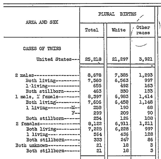
With a few reasonable assumptions, we can use this data to compute the probability that Elvis was an identical twin, given that his twin brother died at birth.

You can see my solution in this Jupyter notebook.

Among U.S. college students, religious attendance is at an all-time low

In the last 30 years, college students have become much less religious. The fraction who say they have no religious affiliation tripled, from about 10% to 30%. And the fraction who say they have attended a religious service in the last year fell from more than 85% to less than 70%.

I’ve been following this trend for a while, using data from the CIRP Freshman Survey, which has surveyed a large sample of entering college students since 1966.

The most recently published data is from “97,753 first-time, full-time students who entered 147 U.S. colleges and universities of varying selectivity and type in the fall of 2018.”

Of course, college students are not a representative sample of the U.S. population. And as rates of college attendance have increased, they represent a different slice of the population over time. Nevertheless, surveying young adults over a long interval provides an early view of trends in the general population.

Religious preference

Among other questions, the Freshman Survey asks students to select their “current religious preference” from a list of seventeen common religions, “Other religion,” “Atheist”, “Agnostic”, or “None.”  

The options “Atheist” and “Agnostic” were added in 2015.  For consistency over time, I compare the “Nones” from previous years with the sum of “None”, “Atheist” and “Agnostic” since 2015.

The following figure shows the fraction of Nones from 1969, when the question was added, to 2018, the most recent data available.

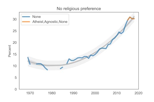Percentage of students with no religious preference from 1969 to 2018.

The blue line shows data until 2015; the orange line shows data from 2015 through 2018. The gray line shows a quadratic fit.  The light gray region shows a 90% predictive interval.

Since 2015, the total fraction of atheists, agnistics, and Nones has been essentially unchanged. The most recent data point is below the trend line, which suggests that the “rise of the Nones” may be slowing down.

Attendance

The survey also asks students how often they “attended a religious service” in the last year. The choices are “Frequently,” “Occasionally,” and “Not at all.” Respondents are instructed to select “Occasionally” if they attended one or more times, so a wedding or a funeral would do it.

The following figure shows the fraction of students who reported any religious attendance in the last year, starting in 1968. I discarded a data point from 1966 that seems unlikely to be correct (66%).

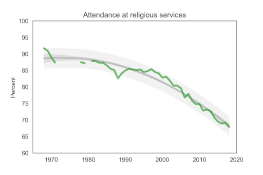Percentage of students who reported attending a religious service in the previous year.

About 68% of incoming college students said they attended a religious service in the last year, an all-time low in the history of the survey, and down more 20 percentage points from the peak.

In contrast with the fraction of Nones, this curve is on trend, with no sign of slowing down.

In previous years I have also reported on the gender gap in religious affiliation and attendance, but the data are not available yet. I will update when they are.

Data Source

The American Freshman: National Norms Fall 2018
Stolzenberg, Eagan, Romo, Tamargo, Aragon, Luedke, and Kang,
Higher Education Research Institute, UCLA, December 2019

This and all previous reports are available from the HERI publications page.

Young Christians are more sex-positive than the previous generation

This is the fifth and probably final in a series of articles where I use data from the General Social Survey (GSS) to explore

Differences in beliefs and attitudes between Christians and people with no religious affiliation (“Nones”),Generational differences between younger and older Christians, andGenerational differences between younger and older Nones.

In the first article, I looked at changes in religious beliefs and found that younger Christians are more secular in many ways than the previous generation.

In the second article, I looked at views related to law and public policy and found that young Christians are more progressive on most issues than the previous generation.

In the third article, I found that generational differences on most questions related to abortion are small and probably not practically or statistically significant.

In the fourth article, I looked at responses to questions related to priorities and public spending. On many dimensions, younger Christians are moving toward the beliefs of their secular peers, but there are notable exceptions.

In this article, I use the same dataset to explore changes in attitudes related to sex. For details of the methodology, see the first article.

When is sex wrong?

GSS respondents were asked several questions related to their attitudes about sex:

There’s been a lot of discussion about the way morals and attitudes about sex are changing in this country.

If a man and woman have sex relations before marriage, do you think it is always wrong, almost always wrong, wrong only sometimes, or not wrong at all?What if they are in their early teens, say 14 to 16 years old? In that case, do you think sex relations before marriage are always wrong, almost always wrong, wrong only sometimes, or not wrong at all?What about sexual relations between two adults of the same sex–do you think it is always wrong, almost always wrong, wrong only sometimes, or not wrong at all?What is your opinion about a married person having sexual relations with someone other than the marriage partner–is it always wrong, almost always wrong, wrong only sometimes, or not wrong at all?

For each of these questions, I count the fraction of respondents who reply “always wrong”.

And I looked at responses to one other sex-related question:

Would you be for or against sex education in the public schools?

Here are the results:

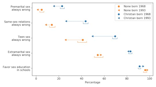Generational changes in attitudes related to sex.

The blue markers are for people whose religious preference is Catholic, Protestant, or Christian; the orange markers are for people with no religious affiliation.

For each group, the circles show estimated percentages for people born in 1968; the arrowheads show percentages for people born in 1993.

For both groups, the estimates are for 2018, when the younger group was 25 and the older group was 50. The brackets show 90% confidence intervals.

In almost every scenario, young Christians are less likely than the previous generation to say that sex is “always wrong”, and in the cases of homosexual and teen sex, the changes are substantial.

Opposition to premarital sex was already low and did not change as much. Support for sex education was already high and is now an overwhelming majority.

The exception is extramarital sex, where there is practically no generational change: more than 80% of both generations think it is always wrong.

Compared to their Christian peers, the non-religious are more sex-positive by 15-30 percentage points. And their generational changes go in the same direction, with young Nones less likely to think sex in these scenarios is wrong.

But again, extramarital sex is the exception; among the Nones, the small generational change is within the margin of error.

This exception suggests that both groups distinguish between actions that harm people and transgressions of divine law.

Summary

In 2007, when I started writing about religious trends, I thought the increasing number of people with no religious affiliation was hugely underreported. Now, the “rise of the Nones” is well known.

Then, for a while, the story was that people were leaving organized religion, but they were still religious or at least spiritual; that is, they were “believing without belonging”.

More recently, it has become clear that beliefs and attitudes among the Nones are getting more secular.

In this series of articles, I have looked at changes among the ones who are left behind; that is, the decreasing fraction who identify as Christian. On many dimensions, the pattern is the same: young Christians are more secular than the previous generation.

Responses that follow this pattern include:

Almost all religious beliefs and activities, except belief in the afterlife.Opposition to sex and sex education, except extramarital sex.Matters of public policy including the legalization of marijuana, pornography, and euthanasia; support for affirmative action; and opposition to the death penalty and school prayer.

Many questions related to public spending follow the same pattern, with younger Christians generally moving toward positions held by their secular peers; the only substantial exception is mass transportation, which has less support among young people in both groups [although this result is so surprising to me that I need more evidence to be confident it is correct].

The most notable exceptions are opposition to gun control and abortion, which show almost no generational changes. Maybe not coincidentally, these exceptions are probably the most politicized topics among the questions I explored.

In summary, we can describe secularization in the U.S. as the sum of two trends, changes in affiliation and changes in belief. Both trends are moving fast, and they are moving in the same direction, away from religion.

Generational changes in public spending priorities

This is the fourth in a series of articles where I use data from the General Social Survey (GSS) to explore

Differences in beliefs and attitudes between Christians and people with no religious affiliation (“Nones”),Generational differences between younger and older Christians, andGenerational differences between younger and older Nones.

In the first article, I looked at changes in religious beliefs and found that younger Christians are more secular in many ways than the previous generation.

In the second article, I looked at views related to law and public policy and found that young Christians are more progressive on most issues than the previous generation.

In the third article, I found that generational differences on most questions related to abortion are small and probably not practically or statistically significant.

In this article, I use the same dataset to explore changes in opinions about public spending and national priorities. For details of the methodology, see the previous article.

Public spending priorities

GSS respondents were asked, “We are faced with many problems in this country, none of which can be solved easily or inexpensively. I’m going to name some of these problems, and for each one I’d like you to tell me whether you think we’re spending too much money on it, too little money, or about the right amount.”

Since they asked about 18 areas of public spending, I’ve put them in three categories:

Areas where young people are more inclined to increase spending,Areas where young people are less inclined to increase spending, andAreas where generational differences are inconsistent or small.

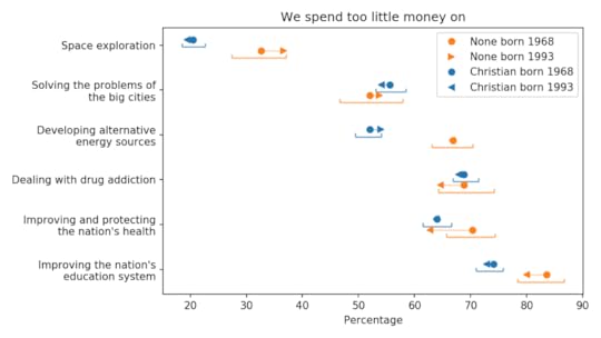
The following figure shows the first group, areas where young people are more likely to say we spend too little:

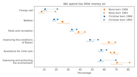Generational changes in views on public spending

The blue markers are for people whose religious preference is Catholic, Protestant, or Christian; the orange markers are for people with no religious affiliation.

For each group, the circles show estimated percentages for people born in 1968; the arrowheads show percentages for people born in 1993.

For both groups, the estimates are for 2018, when the younger group was 25 and the older group was 50. The brackets show 90% confidence intervals.

The way these questions were posed, I suspect that most respondents can’t answer them literally. Few people know how much we spend in each area, what we spend it on, or what effect it would have if we spent more.

So their answers reflect some combination of how important they consider each issue, how much they think we are spending, and how effective they imagine more government spending would be.

With those caveats, we can draw a few conclusions:

On these issues, the priorities of Christians and Nones are generally aligned. The biggest difference between the groups is on spending to protect the environment, but a majority of both groups think we are spending too little.The biggest generational changes are in foreign aid and protecting the environment; on both issues, young people are substantially more inclined to increase spending. But with respect to foreign aid, it is still a small minority.

The following figure shows areas of public spending where the generational change is generally negative:

Generational changes in views on public spending

Compared to their parents’ generation, young people are substantially less likely to increase spending on the military, transportation infrastructure and Social Security. To me, the direction of those changes is not surprising, but the magnitude is.

The other change I find surprising is in support for mass transportation, which decreased in both groups. I double-checked the data and this result seems to be correct, but it might warrant more investigation.

Finally, the following figure shows areas of public spending where generational changes are small and unlikely to be practically or statistically significant.

Generational changes in views on public spending

On these issues, the spending priorities of Christians and Nones are generally aligned, although Nones are more inclined to increase spending on space exploration, alternative energy, and education.

In the next article, I’ll look at generational changes related to confidence in various government and private institutions.

A large majority of Americans support legal abortion, at least in some circumstances

This is the third in a series of articles where I use data from the General Social Survey (GSS) to explore

Differences in beliefs and attitudes between Christians and people with no religious affiliation (“Nones”),Generational differences between younger and older Christians, andGenerational differences between younger and older Nones.

In the first article, I looked at changes in religious beliefs and found that younger Christians are more secular in many ways than the previous generation.

In the second article, I looked at views related to law and public policy and found that young Christians are more progressive on most issues than the previous generation.

In this article, I use the same dataset to explore changes in opinions about abortion. For details of the methodology, see the previous article.

GSS respondents were asked, “Please tell me whether or not you think it should be possible for a pregnant woman to obtain a legal abortion” under different circumstances.

The following figure shows the results.

Generational changes in beliefs about legal abortion

The blue markers are for people whose religious preference is Catholic, Protestant, or Christian; the orange markers are for people with no religious affiliation.

For each group, the circles show estimated percentages for people born in 1968; the arrowheads show percentages for people born in 1993.

For both groups, the estimates are for 2018, when the younger group was 25 and the older group was 50. The brackets show 90% confidence intervals.

Before we look for generational changes, we should notice the starting point: a large majority of Americans support legal abortion, at least in some circumstances.

In cases of severe birth defects and pregnancy due to rape, the majority is about 70% of Christians and 90% of the nonreligious.In cases of serious danger to the woman’s health, it’s almost 90% of Christians and nearly all of the nonreligious.

Under other circumstances, opinions are more divided, with support near 40% among Christians and 70% among the Nones.

Looking now at the generational changes, I see only one that is likely to be practically and statistically significant: younger people in both groups are less likely than the previous generation to support legal abortion if there is a chance of serious birth defect.

Even so, there is majority support in both groups, more than 60% among Christians and 80% among Nones at age 25.

In summary:

Beliefs about abortion depend substantially on the circumstances; In many circumstances, a large majority of Christians and the non-religious support legal abortion;Even where there is disagreement between the groups, there is substantial diversity of opinion within both groups;Generational changes in these opinions are generally small and within the statistical margin of error.