Menzie David Chinn's Blog, page 41

(Not) The Leader of the Pack, Again: Wisconsin and Her Neighbors

Political Calculations criticizes me for comparing Wisconsin economic performance against Minnesota, but not other neighbors.

Normally, we’re entertained by Chinn’s analysis, since it frequently involves comparisons of the job growth between Wisconsin and its western neighbor Minnesota since Walker was sworn into office in January 2011, which we find funny because of all the states surrounding Wisconsin, the composition of Wisconsin’s economy is much less similar to Minnesota than it is to any of the states with which the state shares waterfront footage on Lake Michigan, which is something that one might think an economics professor at the University of Wisconsin-Madison would know.

Gee, I think I’d done this comparison, somewhere in the dim past. Oh, it was August 20, 2014, a full five months ago. In Figure 2 of that post, Wisconsin lagged all her neighbors.

Perhaps the choice of states was in dispute. I used adjoining states; Political Calculations appears to favor the region defined by this map (Census region Great Lakes).

Source: Political Calculations (February 26, 2015).

So, let’s examine the relative performance of Wisconsin against the neighbors, defined by Political Calculations. (Side note: Ohio does not have waterfront on Lake Michigan.)

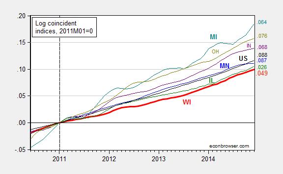
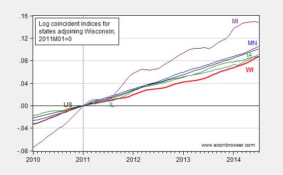
Figure 1: Log coincident indices for Wisconsin (bold red), Minnesota (blue), Illinois (green), Michigan (teal), Indiana (purple), Ohio (chartreuse), United States (black), all normalized to 2011M01=0, seasonally adjusted. Numbers on right hand side (color coded) refer to log-differences relative to NBER defined peak of 2007M12. Source: Philadelphia Fed, and author’s calculations.

If my eyes do not deceive, the bold red line (Wisconsin) lies below all other series. Had I included Kansas, well, you know where that state’s index would lie. (Hint: as of December, it is 1.5 percentage points below that of Wisconsin’s.) As indicated in the notes to Figure 1, the Philadelphia Fed data are readily available for download in Excel spreadsheet should one want to check my calculations.

More on other indicators, from Flavelle/Bloomberg View.

Oh, here is the latest on the Quarterly Census on Employment and Wages, which astute readers will recall (e.g., here) is the series that Governor Walker was for before he was against: Wisconsin’s job creation remained sluggish in latest 12-month report:

Turning in another laggard job-creation report, Wisconsin gained 27,489 private-sector jobs in the 12 months from September 2013 to September 2014, according to data released Tuesday by the state Department of Workforce Development.

The QCEW is a census while the BLS household survey series that Political Calculations displays in this graph is based on a survey (I think; the graph identifies the source as Census, while I have an identical series that is sourced from BLS). That is why the Walker Administration originally favored the QCEW over the establishment survey (Apparently that viewpoint is now “inoperative”, since I no longer hear the QCEW lauded by Walker administration officials.)

So, in summary, the data I have indicate that Wisconsin’s economic performance since 2011M01 has been lackluster. I would welcome actual data indicating otherwise. (Side question: Why are almost every series plotted in the Political Calculations post reporting in nominal terms? The sole exception is tax collections per employee, which would seem to drift upward over time with real per capita income. Curious and curiouser…)

Working with Qualitative Variables: Correlation, Causation, and Third Factors

I am fascinated by maps, including maps of the United States which display the geographic variation of institutional features. But qualitative features, such as institutions or laws, cannot be directly subjected quantitative analysis. Fortunately, as I’ve been discussing in my intro econometrics class, one can convert qualitative data into quantitative data by use of dummy variables, i.e., variables that take on a value of 1 or 0 (one could have ordinal values as well, but I’ll skip that aspect today).

These four maps depict qualitative data applying to the 50 states plus the District of Columbia, to yield 51 observations. Blue means presence of the relevant institutional feature, gray means absence. I’ll consider four such features, call them Z1, Z2, Z3, and Z4.

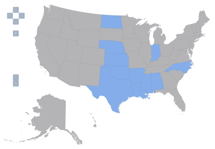
Figure 1: United States, variable Z1=1 denoted by blue, variable Z1=0 by gray.

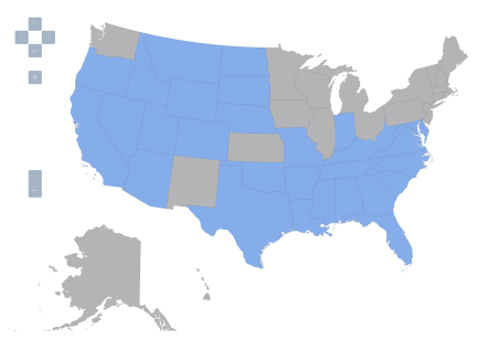
Figure 2: United States, variable Z2=1 denoted by blue, variable Z2=0 by gray.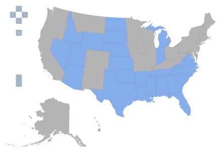






Figure 3: United States, variable Z3=1 denoted by blue, variable Z3=0 by gray.

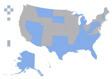
Figure 4: United States, variable Z4=1 denoted by blue, variable Z4=0 by gray.

Notice the interesting pattern. I convert the categorical data in these four maps into quantitative data using dummy variables, Z1 through Z4. Here are the correlation coefficients for the four variables, along with associated t-stats for the null hypothesis the correlation coefficient is zero.

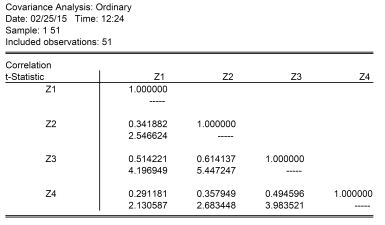
Notice the correlation between Z2 and Z3 are the highest, at 0.61. The t-statistic for the null of zero correlation coefficient is soundly rejected at any conventional significance level. This confirms the impression gained by a visual inspection of maps 2 and 3; however, now we have a quantitative measure. (Note that the interpretation of a Pearson correlation coefficient when applied to binary variables is as a phi coefficient, also referred to as the “mean square contingency coefficient”.)

One can examine how the states align along each dimension by looking at a contingency table for Z2 and Z3 (notice the “phi coefficient” is the same as the correlation coefficient).

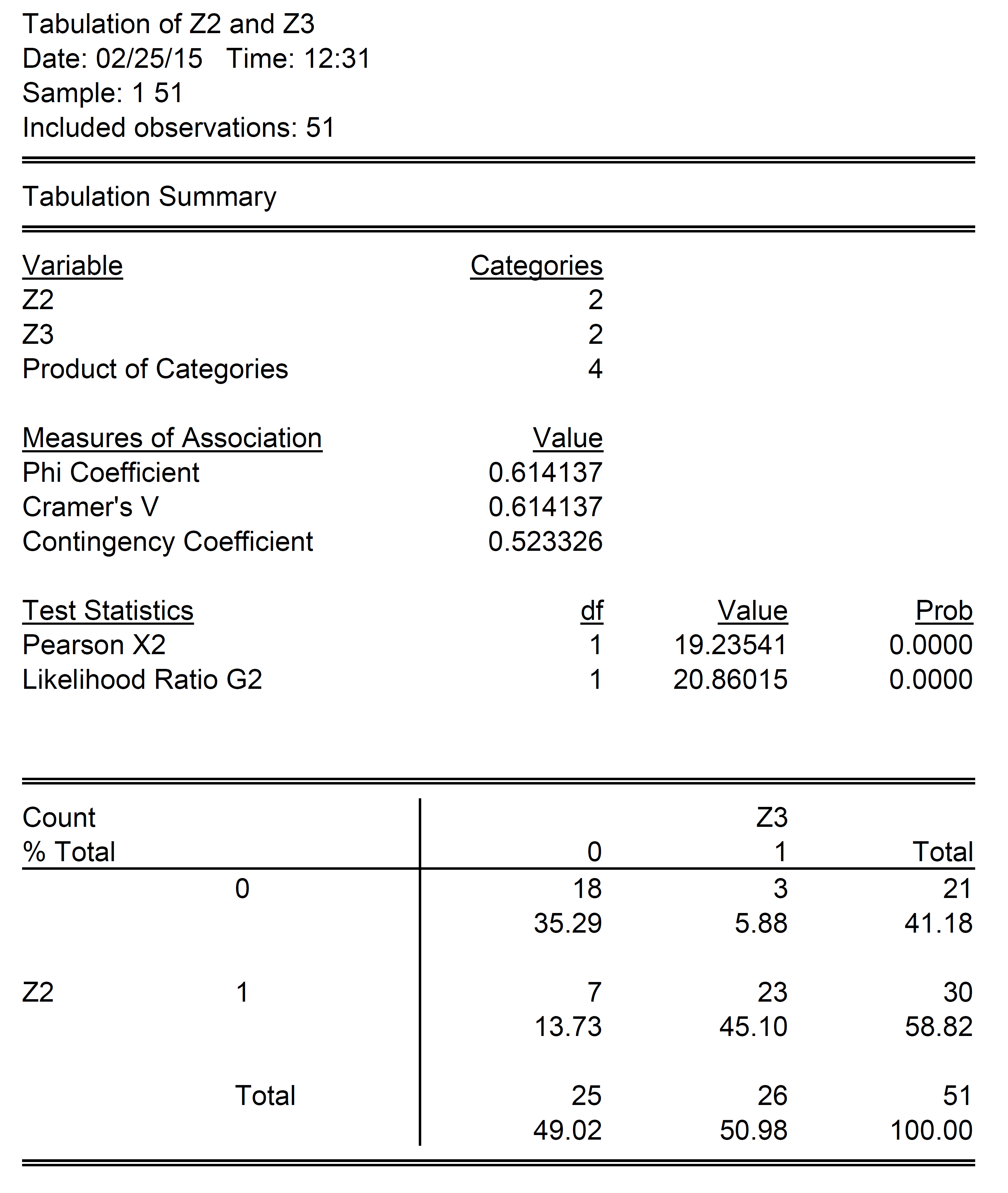
Eighteen states (35.3% of sample) fail to exhibit both of the characteristic in Z2 and Z3, while 23 states (45.1% of sample) exhibit both of the characteristic in Z2 and Z3. A total 10 states fall “off-diagonal”, with states exhibiting one, and not the other. That is, the correlation is not perfect.

One could estimate a linear regression between Z3 and Z2; this is called a linear probability model. Doing so would yield a slope coefficient of 0.62, adjusted R-squared of 0.36. This means a one unit increase in Z2 would increase the probability of Z3=1 from 0 to 0.62. A linear probability model is problematic to the extent that it does not restrict probabilities to lie between 0 and 1. A probit model, which allows for a nonlinear relationship between Z3 and Z2 (and is based on the cumulative normal distribution) yields the following results:

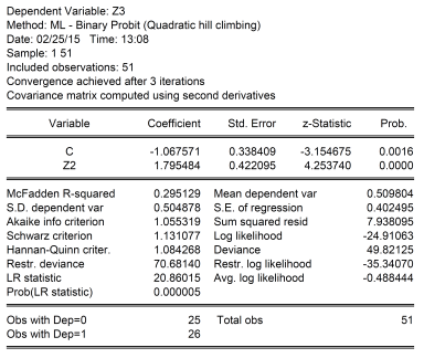
The slope cannot be directly interpreted; one can find the implied probability using the cumulative normal distribution. When Z2 takes on a value of 0, then the probability of Z3=1 is 14.3%. When Z2 takes on a value of 1, then the probability is 76.7%.

Of course, even when one runs a regression, one can’t necessarily say one has identified a causal relationship, regardless of whether the coefficient is statistically significant or not. But certainly, knowing Z2 improves ones guesses of what Z3 will be. In fact, the above probit regression correctly predicts over 68.3% of the cases where Z3 takes on values of 0, and 88.5% of the cases where Z3 takes on values of 1 (assuming a cutoff value of 0.5, that is when the probability Z3=1 exceeds 0.5, predict Z3=1).

To highlight the non-causality interpretation, let’s consider what Z2 and Z3 are. Z3 takes on values of 1 if “right-to-work” laws are in effect, according to the National Right to Work Legal Defense Foundation, Inc.. Z2 takes on a value of 1 if anti-miscegenation laws were in effect in 1947. [1] A causal interpretation would be “having anti-miscegenation laws in 1947 cause one to have right-to-work laws in 2014”; this is clearly implausible. Reverse causality seems also implausible – that is it doesn’t seem likely that “having right-to-work laws in 2014 caused a state to have anti-miscegenation laws in 1947.” It is possible that adding in additional covariates would make the correlation disappear; but if it didn’t, a plausible interpretation is that there is a third, omitted, variable that caused certain states to have anti-miscegenation laws on the books in 1947, and caused certain states to have right-to-work laws in place in 2014.

By the way, the other variables are as follows: Z1 is a dummy variable that takes a value of 1 if restrictions on abortion at 20 weeks are in effect. [2] (some states have restrictions at 24 weeks, some third trimester, yet others at viability; and some had no restrictions.) I wanted to obtain a more general measure of restrictiveness on reproductive rights, but that would have entailed a lot more data collection, so I settled for this dummy variable. Finally, Z4 takes on a value of 1 if the state has implemented “stand-your-ground” laws. [3] Inclusion of these additional variables does not eliminate the statistically significant correlation found in the probit regression equation.

So…correlation is not causation!

Guest Contribution: “1997: The Relevant Threshold in the US Current Account”

Today we are fortunate to have a guest contribution written by Roberto Duncan, assistant professor of economics at Ohio University.

In spite of the current account reversals observed in advanced countries, global imbalances are still a matter of concern (IMF, 2014). Probably, the US current account is the most important component of such worldwide imbalances. The size of the US external deficit has been an issue of analysis for many years. Research on this specific topic has used, at least, two approaches. On the one hand, some researchers contend that thresholds in the dynamics of the current accounts exist. The simplest threshold model can be understood as one where a threshold value is used to identify ranges of values where the behavior predicted by the model varies in some relevant way. For example, Clarida, et al. (2005) find two thresholds in the US current-account-to-GDP ratio. According to that, if the current account surplus is above 2.2% or below -2.2% of GDP, we should expect a reversal toward its long-run mean. Usually, these papers employ only the information contained in the time series of the current account itself (a univariate approach). On the other hand, a number of works based on dynamic stochastic general equilibrium (DSGE) models suggest that the US current account is driven by shocks of fiscal balance, productivity level, productivity volatility, or oil prices.1

Even though a nonlinear univariate model might be useful –for example, for forecasting purposes– its nature leaves aside the fundamentals behind the current account dynamics. The DSGE literature, in turn, usually focuses on linear(ized) relationships and emphasizes one or two factors –partly due to the curse of dimensionality. In the paper titled “A Threshold Model of the US Current Account”, I aim to bridge the gap between these two branches in a multivariate nonlinear framework that can offer more tractability. I address several questions: What are the main drivers of the US current account? Is the behavior of the current account the same during deficits and surpluses or does the size of the external imbalance matter as some analysts suggest? Is there a threshold relationship between the current account and its drivers?

To answer these questions, I estimate a threshold model with multiple regressors to explain the behavior of the US current account during the period between 1973.I and 2012.I, and test for the presence of regimes in its dynamics. As threshold candidates, I try a set of variables suggested by commentators and previous empirical works: the (lagged) level and the size of the current account-to-GDP ratio, the (lagged) level and the size of the fiscal-balance-to-GDP ratio, and time. In the latter case, I actually test for the presence of an unknown time break in the relationship between the regressors and the dependent variable. As regressors, I evaluate a similar set to the one proposed in the DSGE literature mentioned above. In addition, I include the real interest rate and the real exchange rate.2

To deal with the potential endogeneity of the regressors, I use the IV estimator of a threshold model developed by Caner and Hansen (2004).

Main findings

First, in contrast to the univariate threshold models, time is the most important threshold variable. I find a robust time break –not previously documented in the literature– in the relationship between the current account and its main drivers in the third quarter of 1997. Our estimates stubbornly point to 1997.III as the time break even if I use a larger sample such as 1957.I-2012.I.

The time break found in 1997.III coincides with two events: the onset of the Asian financial crisis and the Taxpayer Relief Act of 1997. The former implied a recomposition of portfolios among international investors, including central banks, and the decision of sharp devaluations, the imposition of capital controls, and reserves buildup by monetary authorities. In addition, the Asian financial crisis is viewed as the onset of a sequence of international crises among emerging market economies. Other economies that faced similar crises were Russia (1998), Brazil (1998), Argentina (1999-2002), and Turkey (2001). All of them involved sharp devaluations, modification of the exchange rate regime, and the rise of foreign exchange reserves as a hedge against potential speculative attacks or another financial crisis. While the change in exchange rate policies to limit currency appreciations has led to some to talk about a revived Bretton Woods system (Dooley et al., 2003), the war chests of foreign reserves have, at least in part, led to an increasing purchase of US treasury bonds, which is usually linked to the so- called global saving glut hypothesis (Bernanke, 2005). The second factor that might have contributed to the structural change originated domestically. The Taxpayer Relief Act of 1997, enacted on August 5th, reduced several federal taxes, provided some tax exemptions, and extended tax credits. According to estimates posted by the NBER, the average marginal tax on long-term gains was reduced by almost 7%, from 25.6% to 18.7% in 1997, the largest cut since 1960.

Second, as opposed to what other authors contend, I did not find evidence on the importance of the size or the sign of the current account as threshold variables. The time line always dominates any potential threshold variable previously used or proposed by the empirical literature in terms of model fit. The other candidate variables not only fail to provide an adequate fit compared to the time line, but also they are highly sensitive to the sample, and did not provide either precise threshold or coefficient estimates, or statistics that could support a valid model in each regime.

Third, the most significant determinants of the US current account are total factor productivity, the real exchange rate, the fiscal surplus, and the volatility of productivity in both regimes (before and after 1997.III). As the paper shows, the most statistically significant shifts are related to the productivity level, the real exchange rate, and the real interest rate. In particular, productivity shocks became more important after 1997.

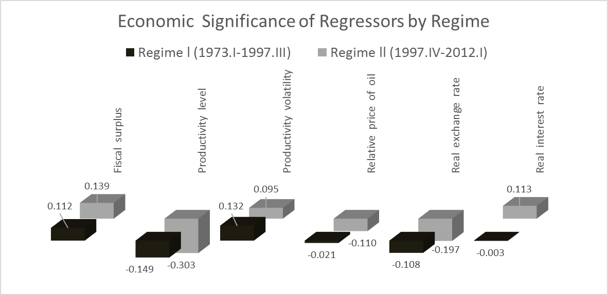
The figure above displays the economic significance of each regressor. That is, the coefficient estimate multiplied by the standard deviation of the corresponding regressor. For example, one-standard-deviation shock in productivity lowers the current account in approximately 0.15 points of long-run GDP in the pre-1997 regime, whereas the respective reduction is 0.3 points of long-run GDP in the post-1997 regime.

Fourth, the relative price of oil and the real interest rate become statistically significant and more economically relevant after 1997, although shocks to these relative prices do not contribute significantly to fluctuations in the current account surplus, at least as much as other regressors of the model. For example, a one-standard-deviation shock in the interest rate would be associated with a rise in the current account of 0.11% of long-run GDP. From an economic viewpoint, the saving glut effect through the interest rate is relatively less important. Similarly, a one-standard-deviation shock in oil prices above its trend would be related to a current account decline of 0.11 percentage points of long-run GDP.

Why did productivity shocks become more important after 1997?

We mentioned that the time break coincides with the onset of the Asian financial crisis. One possibility is that international investors moved their funds from East Asia and, perhaps, other emerging market economies, to the US and invested in more capital-intensive sectors such as the information industry.3 The best example of this investment shift could have been the dot-com bubble observed between 1997 and 2000. The capital intensification of the economy could have made productivity shocks a more important driver of investment and, as a result, the current account. To a lesser degree, another possibility is that the Taxpayer Relief Act of 1997 raised the sensitivity of domestic absorption and, consequently, the sensitivity of the current account to productivity shocks.4

To summarize, we find that time is the best threshold variable in the dynamics of the US current account. In particular, one regime exists before and another one exists after the third quarter of 1997, a period that coincides with the onset of the Asian financial crisis and the Taxpayer Relief Act of 1997. Productivity has become a more important driver of the US current account since then. Further research is needed to verify the reason behind this fact. An important implication for practitioners, who seek to improve the fit of their models that attempt to explain the current account deficit, is the need of taking into account the 1997 structural break and modeling it in a DSGE framework. Such task could be one of the next steps in the research agenda on global imbalances.

References

Acemoglu, D., Guerrieri, V., 2006. Capital deepening and non-balanced economic growth. NBER Working Paper 12475.

Bernanke, B., 2005. The Global Saving Glut and the U.S. Current Account Deficit. Remarks at the Sandridge Lecture, Virginia Association of Economists, Richmond, Virginia. The Federal Reserve Board.

Bodenstein, M., Erceg, C.J., Guerrieri, L., 2011. Oil shocks and external adjustment. J. Int Econ. 83, 168-184.

Bussiere, M., Fratzscher, M., Muller, G., 2010. Productivity shocks, budget deficits and the current account. J. Int. Money Financ. 29, 1562-1579.

Caner, M., Hansen, B., 2004. Instrumental Variable Estimator of a Threshold Model. Economet. Theor. 20, 813-43.

Chinn, M., Prasad, E., 2003. Medium Term Determinants of Current Accounts in Industrial and Developing Countries: An Empirical Exploration. J. Int Econ. 59(1), 47-76.

Clarida, R., Goretti, M., Taylor, M., 2005. Are There Thresholds of Current Account Adjustments? NBER conference G7 Current Account Imbalances: Sustainability and Adjustment.

Dooley, M., Folkerts-Landau, D., Garber, P., 2003. An Essay on the Revived Bretton Woods System, NBER Working Paper No. 9971.

Duncan, R., 2015. A Threshold Model of the US Current Account, forthcoming in Economic Modelling.

Fogli, A., Perri, F., 2006. The Great Moderation and the U.S. External Imbalance. Monetary and Economic Studies (Special Edition). 209-234.

International Monetary Fund, 2014. World Economic Outlook, Legacies, Clouds, Uncertainties (October).

1. See Bussiere, et al. (2010), Fogli and Perri (2006), and Bodenstein, et al. (2011), respectively. Another branch of the empirical literature centers its attention to medium-term fluctuations of the current account using cross-country samples (e.g., Chinn and Prasad, 2003) and overlaps with the DGSE branch. The inclusion of demographic regressors, for example, is more appropriate in cross-country regressions rather than time-series models due to their low variability over time.

2. A reduction in this index indicates real currency depreciation.

3. According to Acemoglu and Guerreri (2006), the information sector in the US has a capital share of 0.53 (the average capital intensity is around 0.4).

4. Consider, for simplicity, an economy in which a productivity shock raises dividends and, therefore, generates capital gains. If capital gains are taxed at the rate t, then consumption would increase by a proportion that depends on 1-t. If such tax rate is reduced, the sensitivity of consumption to productivity shocks would increase.

This post written by Roberto Duncan.

The Congressional Budget Office at 40

The CBO has been providing nonpartisan budgetary and economic analyses for four decades. Whether that continues depends upon the willingness of leaders in Congress believe in the worth of serious analysis (see here for doubts). For now, we look back and (hopefully) forward, at events today. Yesterday, a forum at the Brookings Institution presented some additional views. Director Doug Elmendorf blogs on the anniversary today.

Here’s the program for CBO at 40

Welcome

Douglas W. Elmendorf, Director

Opening Remarks

Representatives of the Budget Committees

Keynote

Alice Rivlin, Founding Director

Panel Discussion

A panel of former Congressional Budget Office directors will discuss CBO’s past and future. The panelists will also respond to questions from the audience.

Alice M. Rivlin, Director 1975-1983,

Senior Fellow, Brookings Institution

Rudolph G. Penner, Director 1983-1987,

Senior Fellow, The Urban Institute

Robert D. Reischauer, Director 1989-1995,

President Emeritus, The Urban Institute

June E. O’Neill, Director 1995-1999,

Professor of Economics, Baruch College

Dan L. Crippen, Director 1999-2003,

Director, National Governors Association

Douglas Holtz-Eakin, Director 2003-2005,

President, American Action Forum

Peter R. Orszag, Director 2007-2008,

Vice Chairman of Corporate and Investment Banking, Citigroup

Closing Remarks

Audit the Fed

Senator Rand Paul (R-KY) has gathered significant bipartisan support for the Federal Reserve Transparency Act of 2015, his proposal for more audits of the Fed. I’ve been trying to understand why any sensible person would think this is a good idea.



Jim Guest says the bill would serve Americans’ “right to know where their tax dollars are going.” Perhaps he meant to say Americans’ right to know where the Treasury’s revenues are coming from rather than where tax dollars are going. The Federal Reserve’s net contributions to the U.S. Treasury have averaged +$83 billion per year since 2009. Last year’s federal deficit would have been almost $100 billion bigger if it had not been for the net positive revenue contributions from the Fed.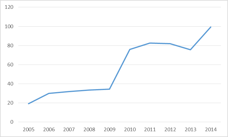

Net receipts of the U.S. Treasury from the Federal Reserve, fiscal years 2005-2014. Data source: Treasury Bulletin.

John Tate thinks the bill would help address “the silent, destructive tax of monetary inflation.” But inflation as measured by the consumer price index has averaged under 1.8% over the last decade. That’s the lowest it’s been since the 1960s.

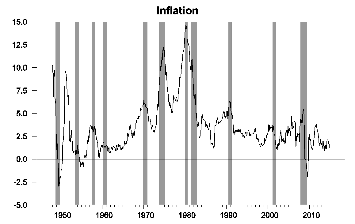
Year over year percent change in consumer price index.

Of course, many of the same people who favor Senator Paul’s bill distrust government-collected inflation data like the CPI. So suppose you look at the private Billion Prices Project, which mechanically collects a huge number of prices each day off the internet. According to BPP, inflation over the last year has been if anything lower than the official numbers.

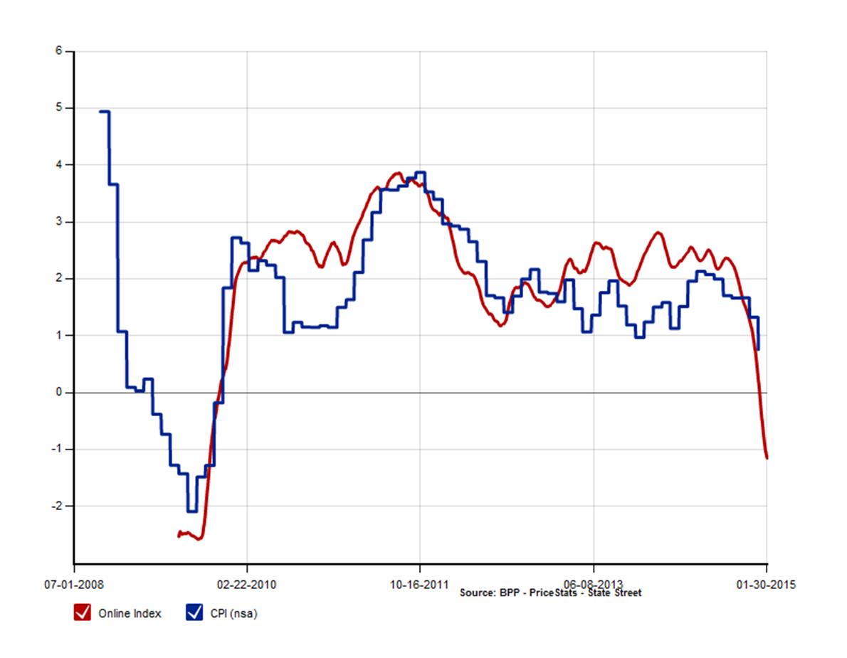
Year-over-year U.S. inflation rate as estimated by BPP (red) and CPI (blue). Source: Billion Prices Project.

Others may take the view that more transparency in and of itself is a good thing. But the Fed is already audited; you can read the audit yourself here. You can examine the Fed’s assets directly down to the level of CUSIP, if you like. Here at Econbrowser we’ve been reporting detailed graphs of the Fed’s assets and liabilities for years using publicly available sources like the weekly H41 statistical release. Cecchetti and Schoenholtz note this conclusion from Richard Fisher, president of the Federal Reserve Bank of Dallas and one of the FOMC’s outspoken critics of quantitative easing:

We are– I’ll be blunt– audited out the wazoo. Every Federal Reserve Bank has a private auditor. We have our auditor of the system. We have our own inspector general. We are audited. What he’s talking about is politicizing monetary policy.

The Wall Street Journal’s David Wessel elaborates:

In 2009, Congress changed the law to allow GAO audits of loans made by the Fed to a single company, such as Bear Stearns or Citigroup, but only when the Fed invoked Section 13(3) of the Federal Reserve Act. (That’s the provision that allows the Fed to lend to almost anybody under circumstances it deems “unusual and exigent.”) The Dodd-Frank law of 2010 further widened the GAO’s authority, allowing it to review the Fed’s internal controls, policies on collateral, use of contractors and other activities—but the GAO is still blocked from reviewing or evaluating the Fed’s monetary-policy decisions.

The Audit the Fed bill would change the law again, and allow the GAO to examine and criticize all monetary policy decisions without restriction.

If we did want to see a lot more inflation for the U.S., Paul’s bill would be the way to get it. The main effect of the bill would be to give Congress an additional tool to exert operational control over monetary policy. The political pressures will be very strong not to raise interest rates when the time does come to start to worry again about inflation. And when the Fed does get to raising rates, it will mean extra costs for the Treasury in paying interest on the federal debt– Congress isn’t going to like that. The primary effect of the legislation would be to give Congress one more stick with which to try to beat up on the Fed when the Fed next does need to take steps to keep inflation from rising.

In fact there’s a pretty dependable historical correlation– the more political control over monetary policy that a country gives to the legislature and the administration, the higher the inflation rate the country is likely to get.

Source: Alesina and Summers (1993) via Cecchetti and Schoenholtz.

Senator Paul’s bill is unambiguously a bad idea.

All the Governor’s Men (Economists)

Paul Krugman notes Governor Walker’s advisers on economics at a recent meeting are Larry Kudlow, Stephen Moore and Arthur Laffer. These folks make appearances in the Econbrowser archives.

Larry Kudlow

From The Financial Crisis: Foreseeable and Preventable (Feb. 2011). Jeff Frieden asks, in the NY Times, why warnings of imminent housing collapse and financial crisis were ignored:

Ideology probably mattered. Larry Kudlow, economics editor of the conservative National Review, in 2005 dismissed “all the bubbleheads who expect housing-price crashes in Las Vegas or Naples, Florida, to bring down the consumer, the rest of the economy, and the entire stock market.” Of course, the bubbleheads were exactly right, but the predictions did not accord with Kudlow’s partisan commitments or his ideology.

And so it is with the post-mortems. Politicians, special interests, and ideologues all have their reasons to insist on a particular interpretation of the crisis. And those connected to the Bush administration have strong incentives to deny that the administration could have done anything differently. But they are wrong.

Stephen Moore

From State Employment Trends: Does a Low Tax/Right-to-Work/Low Minimum Wage Regime Correlate to Growth?, it’s shown that the Laffer-Moore-Williams Rich States, Poor States ranking of business environment does not correlate with growth. 47th ranked California outpaces 17th ranked Wisconsin (or 15th ranked Kansas). Using the entire 50 state ranking, I also show that there is little apparent correlation.

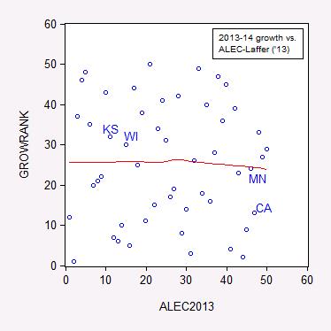
Figure 1: Ranking by annualized growth rate in log coincident index 2013M01-2014M03 versus 2013 ALEC-Laffer “Economic Outlook” ranking. Nearest neighbor nonparametric smoother line in red (window = 0.7). Source: Philadelphia Fed, ALEC, and author’s calculations.

Arthur Laffer

I first met Arthur Laffer more than 30 years ago. His presence on Econbrowser has been consistent, most recently in Whistling past the intellectual graveyard…the Extreme Supply-Sider one in Topeka, that is. Additional appearances, on seasonals (joint appearance with Professor Casey Mulligan), and in spirit, supply side responses (joint appearance with Bill Beach/Heritage Foundation), tax elasticities (joint appearance with Governor Mitt Romney).

I am ever thankful for the likes of Kudlow, Moore, and Laffer, even as they drag down the level of economic discourse. They just provide too many examples of how not to conduct serious analysis.

(For those who don’t recognize the allusion in the title, see here.)

Update, 8PM Pacific:

NB: Rick Stryker Notes that these men are not formally Governor Walker’s economic advisers. That observation is correct; they merely hosted the private meeting that Walker was guest of honor and provided their advice, as discussed here. The Governor has a set of official economic advisers in Wisconsin state government.

Governor Walker Proposes to Restructure Debt Thereby Increasing Total Taxpayer Cost

As the state’s fiscal position becomes more dire, in large part due to the tax cuts implemented last year, Governor Walker proposes to delay some debt payments.

From Jon Peacock at Wisconsin Budget Blog:

We finally learned this week one of the major tactics being used to fill the large hole in this year’s state budget. The Governor plans to push part of the problem further into the future by delaying a $108 million debt payment that is coming due in May.

A Legislative Fiscal Bureau (LFB) memo released yesterday by Reps. Hintz and Taylor explains that there are two kinds of debt restructuring – one that has the effect of reducing the total amount of interest paid on an outstanding debt, and another type that extends the life of an existing debt and increases the total cost to state taxpayers. The planned delay in the $108 million payment is the second type. Although the LFB memo doesn’t show the full impact of the revised payment schedule, it indicates that the delay will increase debt service costs by $544,900 in 2015-16 and more than $18.7 million in 2016-17.

From Yvette Shields in The Bond Buyer:

The [commercial paper] maneuver is fueling Democratic arguments that the state couldn’t afford to tap a budget surplus last year for a $600 million tax cut package. The state faces a $648 million deficit in its next two-year budget. Walker uses spending cuts to deal with the deficit in his proposed $68.2 billion budget.

In other words, no budget repair bill, as when the Governor took office in 2011, [1] but a measure to increase the ultimate debt burden faced by Wisconsin taxpayers.

The Economic Report of the President, 2015

The entire report was released today, covering the “…progress of the recovery and explores the long-term factors that drive middle-class incomes,…the macroeconomic performance of the U.S. economy during 2014, …the opportunities and challenges facing the U.S. labor market, …how American family lives have changed over the last half-century and the implications of these changes for our labor market, …productivity growth with an examination of business tax reform, ..the profound transformation of the U.S. energy sector” and “…the United States in the context of the global economy.”

CEA Chair Jason Furman, CEA Members Maurice Obstfeld, and Betsey Stevenson summarize the report’s findings here.

Guest Contribution: Long-Term Effects of the Great Recession

Today, we’re fortunate to have David Papell and Ruxandra Prodan, Professor of Economics and Clinical Assistant Professor of Economics, respectively, at the University of Houston, as Guest Contributors.

While the Great Recession of December 2007 to June 2009 ended over five years ago, the recovery has been characterized by very slow growth. The Congressional Budget Office has recently released projections of real (inflation adjusted) GDP growth through 2025. If these projections turn out to be correct, real GDP for the U.S. will never return to its pre-Great Recession growth path. This projected decrease in potential GDP is unprecedented, as almost all postwar U.S. recessions, postwar European recessions, slumps associated with European financial crises, and even the Great Depression of the 1930s were characterized by an eventual return to potential GDP.

Suppose you were an econometrician in 2025 and wanted to analyze the long-run effects of the Great Recession. Figure 1 depicts real GDP from 2003:Q3, when potential GDP was re-attained after real GDP returned to its growth path prior to the 2001 recession, through 2025, with actual data through 2014 and projected data thereafter. Figure 1 also depicts the results from estimating a structural change model that allows for one break in the intercept and constrains the growth rate before the break to equal the growth rate after the break. The break, chosen endogenously, occurs in 2008:Q2. This model cannot be rejected in favor of a model where the growth rises after the break until potential GDP is restored and then returns to its pre-break trend.

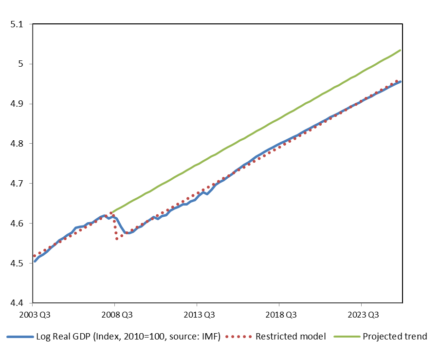
Figure 1: Log real US GDP (2010=100).

In 2011, we presented a paper, “The Statistical Behavior of GDP after Financial Crises and Severe Recessions,” at the Federal Reserve Bank of Boston Conference on the “Long-Term Effects of the Great Recession,” and summarized the results in an Econbrowser post. The focus of the paper was to show that, while severe recessions associated with financial crises generally did not cause permanent reductions in potential GDP, the return takes much longer than the return following recessions not associated with financial crises. We focused on five slumps, extended periods of slow growth and high unemployment, following financial crises identified by Carmen Reinhart and Ken Rogoff in their book, “This Time is Different,” that were of sufficient magnitude and duration to have qualified as comparable to the current Great Slump for the U.S. If the path of real GDP for the U.S. following the Great Recession had been typical of these historical experiences, the Great Slump would have been expected to last about 9 years but would not affect potential GDP. Assuming that the Great Slump started in 2007:4, we predicted that it would not end until 2016:4.

This prediction now appears to be much too optimistic. According to the CBO projections, real GDP will grow by 2.9 percent in 2015 and 2016, 2.5 percent in 2017, and 2.1 percent thereafter. If these projections are correct, potential GDP will never be restored. As shown in Figure 1, while real GDP fell by 4.3 percent from its 2007:Q4 peak to its 2009:Q2 trough, real GDP will permanently be 7.2 percent below the pre-Great Recession growth path because trend real GDP continued to rise during the recession.

In his discussion of our paper at the Boston Fed conference, Jeremy Piger proposed a model of “purely permanent recessions” with a negative intercept break, but no subsequent changes in growth rates. While we were able to reject this model in favor of our chosen models for all five advanced countries that experienced slumps flowing financial crises, future econometricians will not be able to reject his model if the CBO projections turn out to be correct.

Using the same actual and projected data, the CBO expects that the gap between actual and potential GDP to be essentially eliminated by the second half of 2017. Their calculations, however, assume that the growth rate of potential GDP was 1.4 percent per year between 2008 and 2014. In other words, the gap between actual and potential GDP is eliminated, not by faster growth of actual GDP, but by slower growth of potential GDP.

The questions of why growth has been so low since 2009 and what, if anything, can be done to increase growth in the future are both matters of great controversy and beyond the scope of our research. What we can say, however, is that if growth evolves according to the CBO projections, pre-Great Recession potential GDP will never be restored in any meaningful sense. 

This post written by David Papell and Ruxandra Prodan.

Review of Macroeconomics by Charles Jones

This quarter we shifted to a new textbook for teaching undergraduate macroeconomics at UCSD, which is Macroeconomics by Stanford professor Charles Jones. Here are some of my reactions to the book.

At UCSD we now use Jones’s text in a two-quarter sequence for intermediate macroeconomics, with the first quarter covering long-run growth and the second, which I’m teaching this quarter, dealing with economic fluctuations. One of the things I like about the book is that it allows me to teach an empirically oriented course in which I can put more emphasis on the facts and less on stylized theories. Two full chapters are devoted to describing what happened during the Great Recession, which can serve as an extended case study around which much of the course can focus. To my mind that’s the best way to make the course interesting and relevant to students.

One innovation of Jones’s text is that it dispenses completely with the IS-LM framework, replacing it with a formulation that simply puts the central bank’s choice of the nominal interest rate as a starting point for studying the effects of monetary policy. This follows more closely modern theoretical treatments like Woodford (2003) and Romer (2000), is more consistent with how monetary policy is actually implemented, and saves the instructor the embarrassment of centering the theoretical structure on a concept of money demand that completely breaks down in describing the most recent data.

The text expresses more skepticism than many others about the efficacy of fiscal policy as a short-run tool for demand management, and is also unusual in including a serious discussion of long-term budget constraints. Personally that focus suits me well, though in this dimension it’s not a text that would appeal to Paul Krugman.

One certainly has to be impressed by Jones’s skill (almost paralleling Greg Mankiw’s) at finding a way to cut to the heart of very complicated issues and explain them in a very simple way– to read his text is to admire an artist at work. At times I worry though whether all the details left out will be a hindrance for the best students, and found I wanted to supplement the book’s treatment of topics such as the term structure of interest rates, the details of how monetary policy is implemented, and exactly how the “long-run” and “short-run” models are reconciled. What Jones and many instructors will have in mind is a log-linearization around a long-run growth model in which most of the coefficients have been set to zero for simplicity. But the book never communicates exactly what this entails, having for example taken great pains never to even use the term “logarithm”, plotting instead variables on what is called a “ratio scale”, and just introducing key parameters and “shocks” as defined ratios. I ended up following the text as written just taking the various shocks as given objects, but will want to give some thought next time I teach it to see if there’s another way to sketch for the better students exactly what is going on.

Overall, I’m very happy with the switch to the new text, and would encourage any teachers dissatisfied with the macro texts they’ve been using to give it a look.