Working with Qualitative Variables: Correlation, Causation, and Third Factors

I am fascinated by maps, including maps of the United States which display the geographic variation of institutional features. But qualitative features, such as institutions or laws, cannot be directly subjected quantitative analysis. Fortunately, as I’ve been discussing in my intro econometrics class, one can convert qualitative data into quantitative data by use of dummy variables, i.e., variables that take on a value of 1 or 0 (one could have ordinal values as well, but I’ll skip that aspect today).

These four maps depict qualitative data applying to the 50 states plus the District of Columbia, to yield 51 observations. Blue means presence of the relevant institutional feature, gray means absence. I’ll consider four such features, call them Z1, Z2, Z3, and Z4.

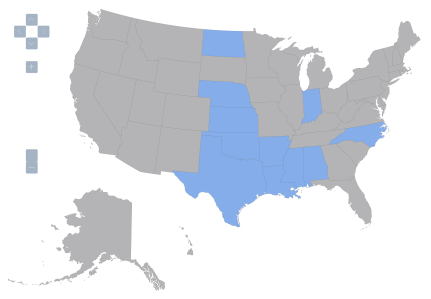
Figure 1: United States, variable Z1=1 denoted by blue, variable Z1=0 by gray.

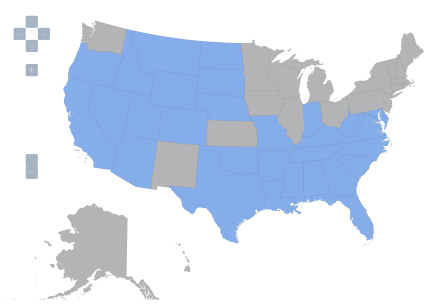
Figure 2: United States, variable Z2=1 denoted by blue, variable Z2=0 by gray.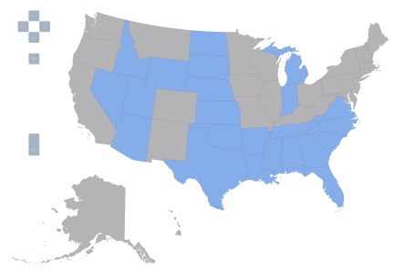






Figure 3: United States, variable Z3=1 denoted by blue, variable Z3=0 by gray.

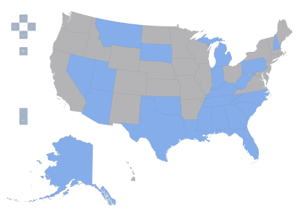
Figure 4: United States, variable Z4=1 denoted by blue, variable Z4=0 by gray.

Notice the interesting pattern. I convert the categorical data in these four maps into quantitative data using dummy variables, Z1 through Z4. Here are the correlation coefficients for the four variables, along with associated t-stats for the null hypothesis the correlation coefficient is zero.

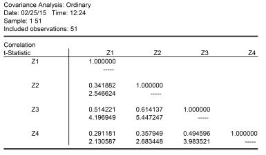
Notice the correlation between Z2 and Z3 are the highest, at 0.61. The t-statistic for the null of zero correlation coefficient is soundly rejected at any conventional significance level. This confirms the impression gained by a visual inspection of maps 2 and 3; however, now we have a quantitative measure. (Note that the interpretation of a Pearson correlation coefficient when applied to binary variables is as a phi coefficient, also referred to as the “mean square contingency coefficient”.)

One can examine how the states align along each dimension by looking at a contingency table for Z2 and Z3 (notice the “phi coefficient” is the same as the correlation coefficient).

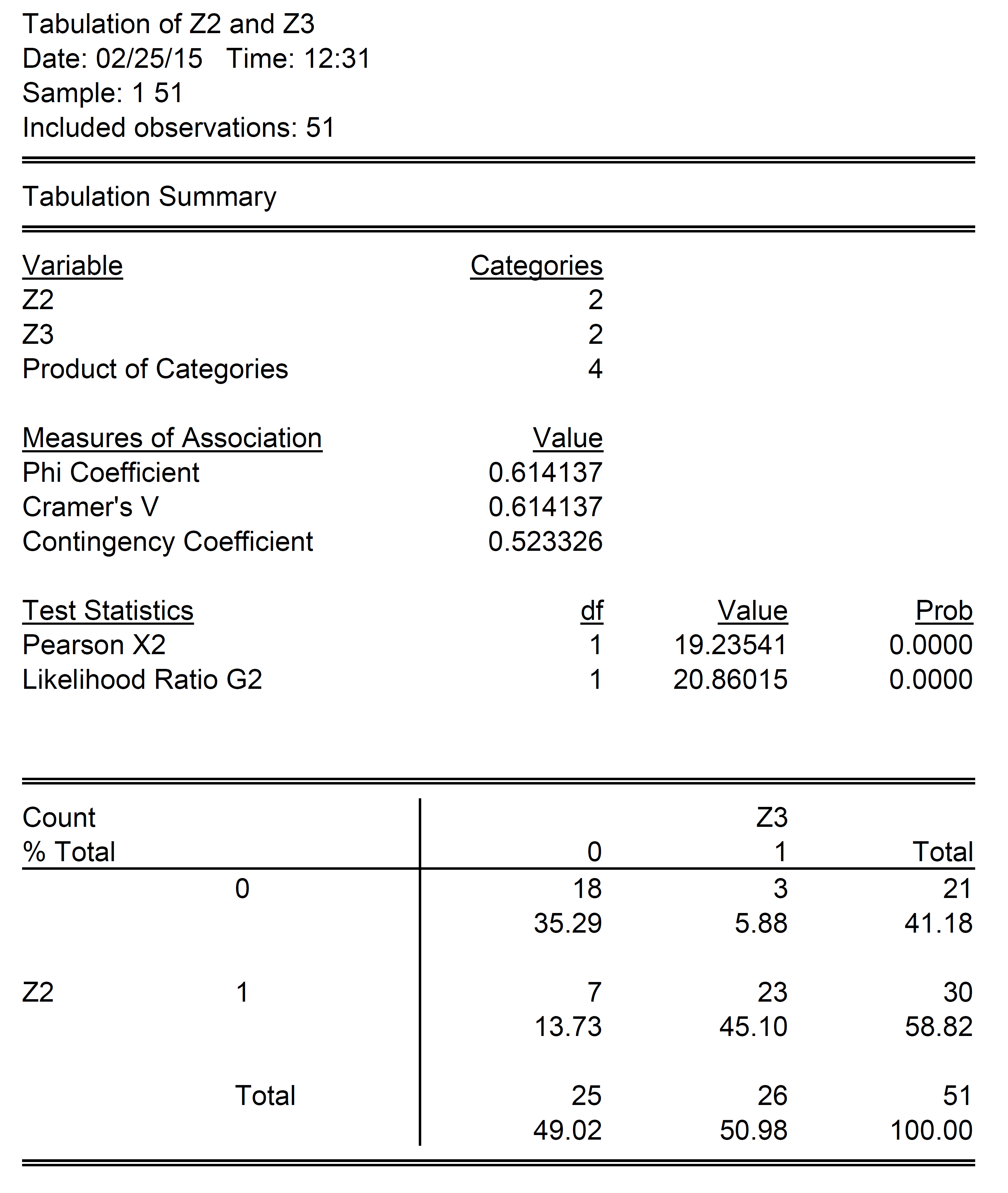
Eighteen states (35.3% of sample) fail to exhibit both of the characteristic in Z2 and Z3, while 23 states (45.1% of sample) exhibit both of the characteristic in Z2 and Z3. A total 10 states fall “off-diagonal”, with states exhibiting one, and not the other. That is, the correlation is not perfect.

One could estimate a linear regression between Z3 and Z2; this is called a linear probability model. Doing so would yield a slope coefficient of 0.62, adjusted R-squared of 0.36. This means a one unit increase in Z2 would increase the probability of Z3=1 from 0 to 0.62. A linear probability model is problematic to the extent that it does not restrict probabilities to lie between 0 and 1. A probit model, which allows for a nonlinear relationship between Z3 and Z2 (and is based on the cumulative normal distribution) yields the following results:

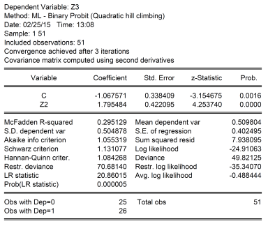
The slope cannot be directly interpreted; one can find the implied probability using the cumulative normal distribution. When Z2 takes on a value of 0, then the probability of Z3=1 is 14.3%. When Z2 takes on a value of 1, then the probability is 76.7%.

Of course, even when one runs a regression, one can’t necessarily say one has identified a causal relationship, regardless of whether the coefficient is statistically significant or not. But certainly, knowing Z2 improves ones guesses of what Z3 will be. In fact, the above probit regression correctly predicts over 68.3% of the cases where Z3 takes on values of 0, and 88.5% of the cases where Z3 takes on values of 1 (assuming a cutoff value of 0.5, that is when the probability Z3=1 exceeds 0.5, predict Z3=1).

To highlight the non-causality interpretation, let’s consider what Z2 and Z3 are. Z3 takes on values of 1 if “right-to-work” laws are in effect, according to the National Right to Work Legal Defense Foundation, Inc.. Z2 takes on a value of 1 if anti-miscegenation laws were in effect in 1947. [1] A causal interpretation would be “having anti-miscegenation laws in 1947 cause one to have right-to-work laws in 2014”; this is clearly implausible. Reverse causality seems also implausible – that is it doesn’t seem likely that “having right-to-work laws in 2014 caused a state to have anti-miscegenation laws in 1947.” It is possible that adding in additional covariates would make the correlation disappear; but if it didn’t, a plausible interpretation is that there is a third, omitted, variable that caused certain states to have anti-miscegenation laws on the books in 1947, and caused certain states to have right-to-work laws in place in 2014.

By the way, the other variables are as follows: Z1 is a dummy variable that takes a value of 1 if restrictions on abortion at 20 weeks are in effect. [2] (some states have restrictions at 24 weeks, some third trimester, yet others at viability; and some had no restrictions.) I wanted to obtain a more general measure of restrictiveness on reproductive rights, but that would have entailed a lot more data collection, so I settled for this dummy variable. Finally, Z4 takes on a value of 1 if the state has implemented “stand-your-ground” laws. [3] Inclusion of these additional variables does not eliminate the statistically significant correlation found in the probit regression equation.

So…correlation is not causation!