Menzie David Chinn's Blog, page 44

Private Employment under Obama and Bush

Reader Move On admonishes me to … move on. So here is job creation in this Administration, in comparative perspective.

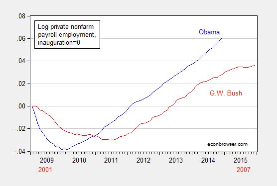
Figure 1: Log private nonfarm private employment normalized to 2009M01 (blue), and to 2001M01 (red). Source: BLS, and author’s calculations.

Figure 2 presents private employment normalized on the relevant troughs (as defined by the NBER).

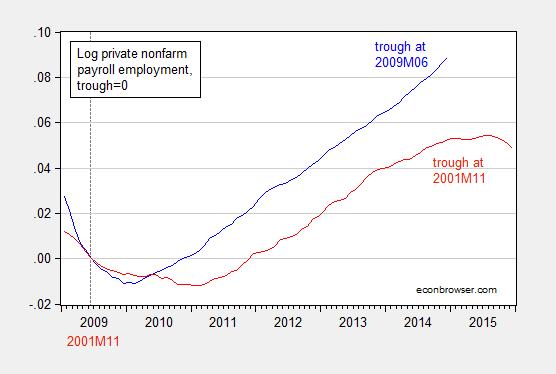
Figure 2: Log private nonfarm private employment normalized to 2009M06 (blue), and to 2001M11 (red). Source: BLS, NBER, and author’s calculations.

The astute observer will note the deceleration in employment growth as one moves toward the end of the G.W. Bush Administration. In fact, private employment was 462,000 less at the end of the G.W. Bush administration than at the beginning, i.e., -0.4% lower (in log terms).

On a related matter, Macroeconomic Advisers and e-forecasting have reported monthly GDP for November and December, respectively. For now, output seems to continue to rise at a fairly rapid clip.

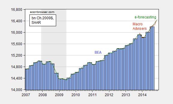
Figure 3: GDP, in billions Ch.2009$, SAAR (blue bars), monthly GDP from Macroeconomic Advisers (red), and e-forecasting (green). NBER defined recession dates shaded gray. Source: BEA 2014Q3 final release, Macroeconomic Advisers (15 Jan.), and e-forecasting (21 Jan.).

Wisconsin: Only 93,200 Net New Jobs Needed in January 2015 to Hit Governor Walker’s 250,000 Jobs Target

According to WI DWD statistics released today.

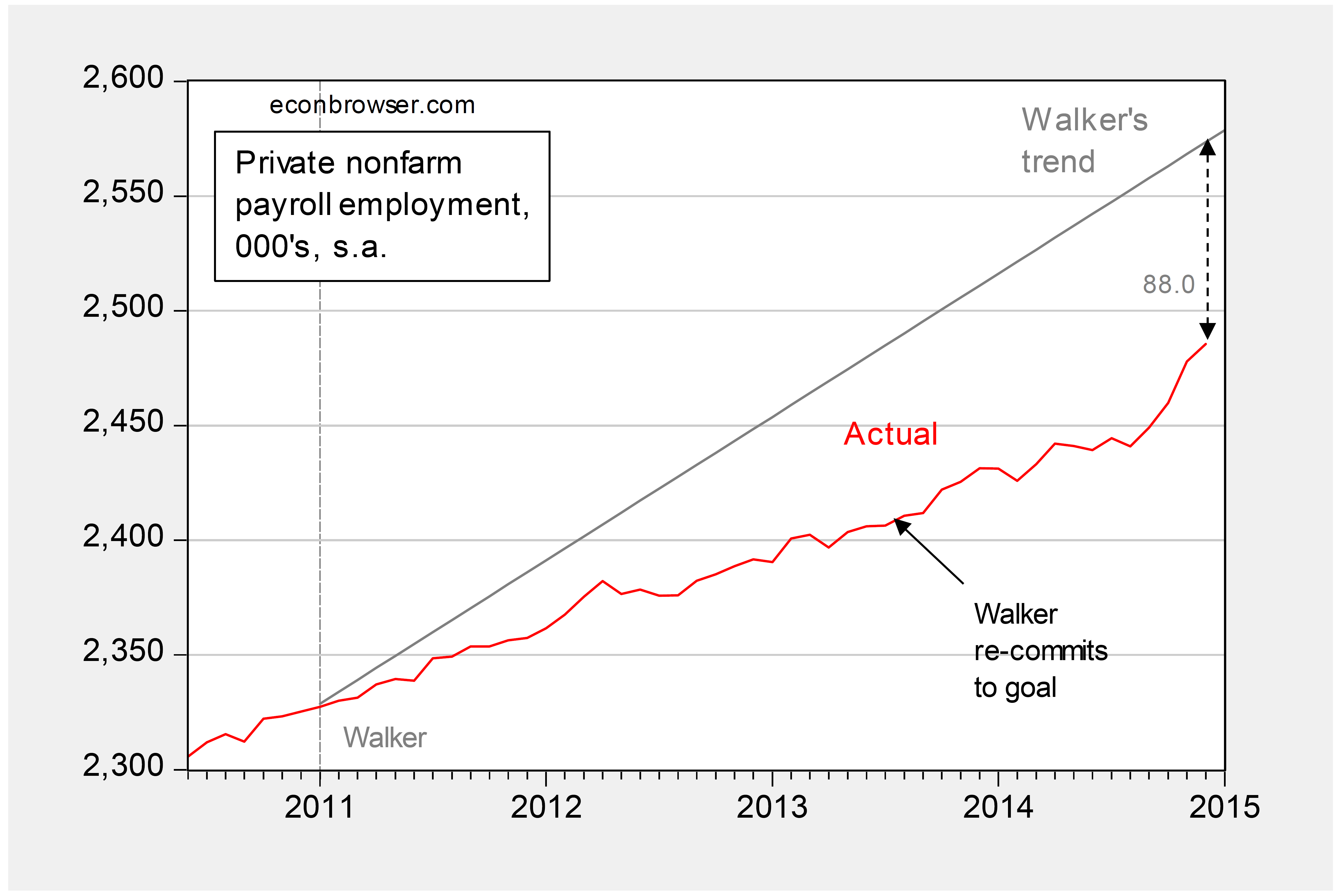
Figure 1: Wisconsin private nonfarm payroll employment (red), and linear trend implied by Governor Walker’s 250,000 net new private sector jobs pledge (gray). Dashed line at beginning of Walker administration. Governor Walker recommits to 250,000 net new jobs in August 2013. Source: WI DWD, Milwaukee Journal Sentinel, and author’s calculations.

Since average net job creation in Wisconsin under Governor Walker has been 3.3 thousand, with a standard deviation of 4.7 thousand, the likelihood that the target will be achieved is low.

But then, as a government official wrote to me on May 16, 2012: “The adminstration assumed that the jobs gains would be back loaded — ramping up with time.” So perhaps the ramp will be extremely steep this month!!!

Figure 2 presents a comparison of Wisconsin’s employment growth against that of the United States.

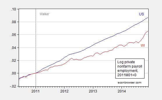
Figure 2: Log private nonfarm payroll employment in US (blue), and Wisconsin (red). Dashed line at beginning of Walker administration. Source: WI DWD, BLS, and author’s calculations.

Guest Contribution: “Measuring the On-going Changes in China’s Capital Controls”

Today we are fortunate to have a guest contribution by Jinzhao Chen (Paris School of Economics) and XingWang Qian (SUNY Buffalo State). This post is based on this paper.

The 2008 financial crisis and the subsequent US Fed’s quantitative easing (QE) policy followed by its “taper” expectation caused wild swings of capital flows across the border of emerging economies. Despite disruptive, many emerging economies, including Brazil, Taiwan, and South Korea, had a successful experience with capital controls to manage volatile capital flows and fended off the contagion (Gallagher, 2011; IMF 2011).

Capital controls are back (Eichengreen and Rose, 2014)! The 2008 global financial crisis opens a new chapter of policy discussion on how to use capital controls to deal with the boom-and-bust capital flows.

Maintaining the primacy of financial liberalization, IMF started to soften its opposition and in 2011 partially recognized the appropriateness of capital control; then in 2012 IMF endorsed it in an institutional view (IMF 2012) and went on to recommend a set of guidance regarding the appropriate use of capital flow management (CFM) (IMF 2013).

China has a history of having recourse to tough regulations on cross-border capital flows, particularly on capital account flows. Tight controls on capital account prevented China from financial instability. For instance, China survived the storm of the 1997 Asian financial crisis. The then US Treasury Secretary Rubin praised China as the “island of stability” in the region. With the capital controls, China seemed to manage the risk of possible contagion from the 2008 global financial crisis well.

Meanwhile in the past decade, China made great efforts to liberalize its capital account to confront some emerging economic challenges, e.g. global imbalance of payment and slowing-down economic growth. PBOC, China’s central bank, outlined a three-stage reform proposal in 2012 to promote the international use of the RMB and to open up China’s capital account in ten years. However, IMF warned via the Wall Street Journal (2013) that speedy liberalization could trigger massive capital exodus if not properly handled. The estimated net outflows from China could be up to 15% of the country’s GDP (Bayoumi and Ohnsorge, 2013) over several years. Domestic banking system may not be resilient enough to withstand such shocks, thus could trigger a financial crisis.

In the paper entitled “Measuring the On-going Changes in China’s Capital Flow Management: A de jure and a Hybrid Index Data Set,” we create a new indices data set measuring the changes in China’s capital controls, expecting that the indices help better study China’s capital controls and assess the process of capital account liberalization and its implications for Chinese economy.

Our monthly indices data are from 1999 to 2012 (due to the availability of AREAER data), and comprised of two groups of indices, de jure and hybrid indices. Both groups include indices created for selected subcategories of China’s capital account, including equities, bonds, money market instruments, commercial credits, financial credits, and FDIs. Further, similar indices are generated from the aspects of controlling on inflows and outflows, resident and nonresident. Given the fact that China’s total imports and exports account for more than 50% of GDP, and that investors could easily move their capitals in and out via, for example, trade mis-invoicing (Cheung and Qian, 2010), we also create indices for China’s control on current account payment flows.

The indices data are compiled by extracting the detailed information from the text of IMF’s Annual Report on Exchange Arrangements and Exchange Restrictions (AREAER). China usually implements policies step by step in the gradualism style, we extract those information of small-step policy measures from the line of the text in IMF’s AREAER and some supplementary materials from other sources. Our goal is to incorporate as detailed and accurate information as possible about China’s capital controls.

Given that we measure the change of intensity in capital controls, we set the level of capital control at January 1999 as the benchmark and give a score of 0. Whenever there is a policy change that tightens the capital control, we add value 1 to the existing score. If there is a control-relaxing policy change, we subtract 1 from the existing score. Otherwise, we keep the score unchanged from the existing one. In this way, the higher score of our indices represents the tighter controls that Chinese government imposes on capital flows.

In comparison to other indices, for instance, Chinn-Ito index, Quinn (1997) and Schindler (2009) index, our indices measure the intensity changes in China’s capital controls over time in monthly frequency, display more variation during the sample period (Figure 1) and contain less subjective judgment.

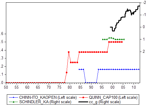
Figure 1: Comparison to other de jure indices

Our indices reveal a persistent but uneven process of liberalizing China’s capital account since 2000. As shown in Figure 2, there is a clear downward trend (a lower index represents a more liberalized capital account) in the gross capital account control index (CC_G). China kept loosening the control grip on its capital account, although there was a temporary reverse over the concern about the spillover of 2008 global financial crisis. The control index for gross flows of current account (CA) also indicates a liberalizing trend, but with a much slower pace than the capital account. Particularly during the period from 2005 to 2008 before the global financial crisis, rather than continuing liberalizing, China stringed up the trade payments controls. It is probably due to the fact that China was using policy tools to deal with the booming trade surplus to ease the political pressure from major trade partners.

In general, the control indices of both current account and capital account move in tandem, revealing that the Chinese government coordinates capital control tools in both current account and capital account. In addition, our indices may well reflect how the government implements capital control policies in response to major economic events and shocks. For instance, in responding to 2008 financial crisis (pinpointed at the collapse of Lehman Brother in Sept. 2008) when capital “flight to quality” from emerging economies, Chinese government encouraged capital inflows by raising QFII cap from $800 million to $1 billion and reduced the lock-up period for certain medium and long-term capital to 3-month from six-month to 1 year; and allowed foreign investors to participate in interbank foreign exchange market. At the same time, China tightened capital outflow measures to strictly enforce QDII cap on the net amount of funds remitted abroad.

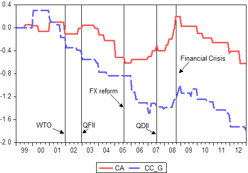
Figure 2: Index of controls on capital account (CC_G) and current account (CA)

References:

Barry Eichengreen, Andrew Rose, 2014 “Capital Controls in the 21st Century,” Journal of International Money and Finance, Volume 48, Pages 1-16

Bayoumi, Tamim and Franziska Ohnsorge, 2013, “Do Inflows or Outflows Dominate? Global Implications of Capital Account Liberalization in China,” IMF Working Paper WP 13/189.

Cheung, Yin-Wong and XingWang Qian, 2010, “Capital Flight: China’s Experience,” Review of Development Economics, Wiley Blackwell, vol. 14(2), pages 227-247, 05.

Chinn, Menzie D. and Hiro Ito, 2008, “A New Measure of Financial Openness,” Journal of Comparative Policy Analysis, Volume 10, Issue 3, p. 309 – 322.

Gallagher, Kevin P. ,2011, “Regaining Control: Capital Controls and the Global Financial Crisis.” Political Economy Research Institute, University of Massachusetts–Amherst.

International Monetary Fund, 2011, “Recent Experiences in Managing Capital Inflows— Cross-Cutting Themes and Possible Policy Framework,” Washington, D.C.: International Monetary Fund.

International Monetary Fund, 2012, “The Liberalization and Management of Capital Flows: an Institutional View,” Washington, D.C.: International Monetary Fund.

International Monetary Fund, 2013, “Guidance Note for the Liberalization and Management of Capital Flows,” Washington, D.C.: International Monetary Fund.

Quinn, Dennis, 1997, “The Correlates of Change in International Financial Regulation,” American Political Science Review, Vol. 91, pp. 531–51.

Schindler, Martin, 2009, “Measuring Financial Integration: A New Data Set,” IMF Staff Papers, Vol. 56. No. 1, pp. 222 – 237.

Wall Street Journal, 2013, “IMF Advises China to Be Cautious With Capital-Account Liberalization.” http://online.wsj.com/news/articles/SB10001424127887324263404578611480166001050 retrieved at Oct. 1, 2014.

This post written by Jinzhao Chen and QingWang Qian.

Guest Contribution: “What Drives Housing Dynamics in China?”

Today we are fortunate to have a guest contribution written by Timothy Bian (University of International Business and Economics, China) and Pedro Gete (Georgetown University).

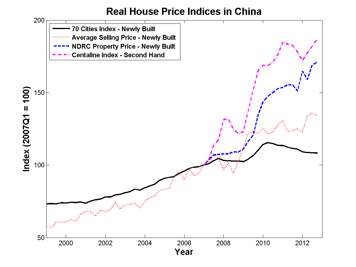
Housing prices in China have increased rapidly. The picture below compares their dynamics with those of the U.S. and other economies.

There is significant heterogeneity among the different indices of Chinese housing prices:

In this paper we analyze five potential drivers of Chinese housing prices:

1. Urbanization and Population Flows.

2. Relaxation of Credit Standards. For example, the shadow banking system. Or financial innovations, such as wealth management products, to circumvent banks’ lending quota.

3. Productivity and Income Growth.

4. Higher Demand for Savings. Real estate is among the few assets available to Chinese households given the capital controls that limit the ability to invest overseas and the non-competitive caps on banks’ deposit rates.

5. Preferences towards Housing. Housing bubbles, or a change in the status value of housing in marriage markets, are two factors that potentially could drive housing demand.

We use SVARs identified with sign restrictions consistent with a standard DSGE model of housing markets. We analyze different indices of housing prices.

Our main results are: 1) The five potential drivers play a non-trivial role in explaining housing prices in China. 2) Productivity growth has been the main driver since 1998. 3) However, when we restrict our data set to the 2007Q1 to 2012Q4 period, then housing preferences, which capture either a bubble or the status value of housing, are the dominant drivers. This result is robust across all price indices. It supports the recommendation from the IMF that China must act to prevent the risks associated with speculative demand in its real estate markets.

This post written by Timothy Bian and Pedro Gete.

IMF World Economic Outlook Update

From the IMF:

Global growth will receive a boost from lower oil prices, which reflect to an important extent higher supply. But this boost is projected to be more than offset by negative factors, including investment weakness as adjustment to diminished expectations about medium-term growth continues in many advanced and emerging market economies.

Here is an excerpt from the update table.

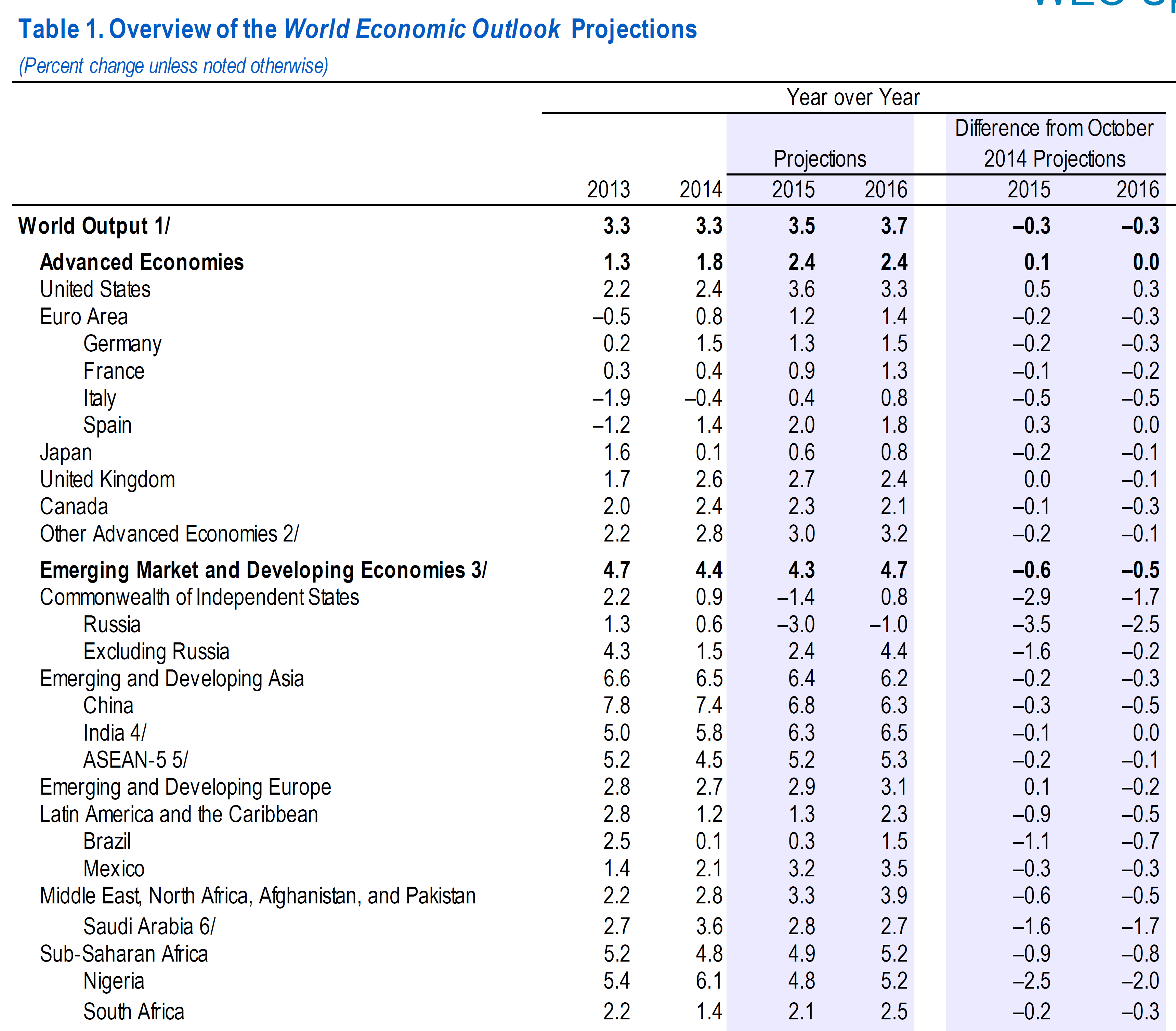
What I find remarkable is the marked deterioration in the prospects for Russia. Year-on-year growth in 2015 and 2016 has been marked down by 3.5 and 2.5 percentage points, respectively, just in the three months since October’s WEO, to -3.0 and -1.0. Growth from 2014Q4 to 2015Q4 is forecasted to be -5.4%. (See this post for discussion of y-o-y vs. 4q/4q growth rates.)

One might speculate that now would be the time to exert maximal leverage via further economic sanctions, should Russia continue to pursue its incursion in eastern Ukraine.

Now some folks (like reader Tom commenting on a similar World Bank forecast) pooh-poohed the magnitude of the implied recession. It’s useful to remind people that the year-on-year drop in the US in 2009 was 2.8%… I think most sensible people think that was a pretty deep recession.

Switzerland drops its currency peg

The Swiss National Bank stunned markets on Thursday with an abrupt decision to abandon its commitment since 2011 to hold the Swiss franc at 1.20 francs/euro, as a result of which the franc appreciated almost 20% within the space of a few minutes.

I have seen some commentators suggest that the Swiss were forced into such a move. Michael Casey wrote:

Ultimately, though, it was again the ECB that foiled the Swiss central bank’s policy. In hinting at a big new bond-buying, or quantitative easing, program, the ECB drove a new, large influx of euros into francs, so many that its Swiss counterpart could no longer keep buying them to maintain the CHF1.20 rate.

And from Bloomberg:

“Nobody, who’s active in the export industry, could expect that the exchange rate of 1.20 per euro would be guaranteed for ever,” economist William White, a former member of the Bank for International Settlements’ executive committee, told Switzerland’s Finanz und Wirtschaft. “The time has come to accept the inevitable.”

I find such claims puzzling. It is one thing to say that a central bank may lack the power to keep its currency value high. Given a finite amount of foreign currency (for example, dollars) that the central bank holds as reserves, it can only buy so much of its own currency with its own holdings of dollars before a speculative attack overwhelms the central bank’s arsenal.

But in this case we’re talking about a commitment from the central bank to keep its currency value low. The policy to implement that calls for buying as many euros as needed, paying for them with francs of which the Swiss can perfectly well create as many as they want all by themselves.

A central bank with the power to create new Swiss francs could hardly claim that it does not have enough francs to buy all the euros that are offered for sale. Here’s the game– you specify a number, and I see if I can make up a bigger number. I should be able to win that game.

If the market is saying the Swiss franc is oh so valuable, oh so desirable, and I have the power to create as many trillions of them as I choose, surely I can change the market’s mind if I try, buying up the entire world, if need be, with Swiss francs that I costlessly create.

Of course, what I could end up doing with such a peg is create inflation. And this is why Lars Svensson proposed a variant of the former Swiss strategy as part of a “foolproof way” to escape deflation and a liquidity trap.

But there appear to be no signs of inflation yet in Switzerland. So why did the Swiss think that the peg could no longer be maintained? I simply do not understand the claim that the central bank was forced to abandon the peg.

I conclude that instead the central bank just wanted to try something different. But I confess that it is a great mystery to me why they wanted to do that. This has to be a major hit to Swiss exports and tourism, leave the Swiss National Bank with little credibility and negative capital, and will likely cause significant financial disruptions in many places around the world.

“Inflation’s Looming Shadow”

Paul Ryan in October 2009 writes:

“One of my key concerns is on the inflation front….”

“…We are already seeing some potentially dangerous developments in financial markets. Over the past six months alone, the dollar has declined nearly 15 percent against major currencies (Figure 4) . Due to extremely low interest rates in the U.S., some investors are using the dollar as a funding currency for a carry trade (borrowing and then selling dollars to buy higher-yielding foreign assets), which is further contributing to downward pressure. A falling dollar pushes up the cost of imported goods and commodities. Gold is at an all-time high above $1,000 per troy ounce (Figure 5) , silver and copper prices are on the rise, and oil prices have doubled over the past 8 months. These commodity price increases could be an early harbinger of future inflation.”

That’s from an op-ed in October 2009. Here are up to date statistics on inflation from today.

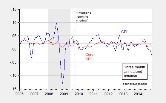
Figure 1: Three month annualized inflation using CPI-all (blue), Core CPI (red). NBER defined recession dates shaded gray. Source: BLS, NBER, author’s calculations.

Hottest on Record

Global temperatures in 2014, that is.

Source: NOAA.

Update, 1/17, 12:45PM Pacific: Since Rick Stryker has asked for statistical significance, but is apparently unable to do statistical testing on his/her own, I will spend some time walking through a quick check.



Download annual data on plotted anomaly, http://www.ncdc.noaa.gov/monitoring-r...

Test for unit root, allowing for constant and trend. You will reject the no unit root null using most versions of the DF test, over entire 1880-2014 sample.

Find the break with the associated lowest p-value/highest significance level in constant, time trend specification; I obtain 1944.

Test for unit root, allowing for constant and trend. You will reject the no unit root null using most versions of the DF test, 1944-2014 sample. You will reject the null, again.

Run a regression of anomaly on constant, time trend; use HAC robust standard errors. I obtain a trend coefficient of 0.01, standard error of 0.001, t-stat for null beta=0 of 9.89.



In my book, that’s enough to reject the null zero-trend hypothesis.

But then, again, Rick Stryker believes 500,000 jobs/month is a typical job creation rate in a recovery!!!! Not true even when one normalizes for labor force, as discussed here. Here’s the rule: When Rick writes, prepare to laugh, and laugh and laugh!!!

Update, 6:45PM: Here is an animation, from that crazy publication, Bloomberg.

The SNB Removes the Cap

Commenting on what has been termed “Francogeddon” and a “tsunami” as well as consequent mayhem, Joe Weisenthal at Bloomberg/Business Week writes:

“Today the Swiss National Bank shocked the world when it announced it would remove the cap it had in place to prevent the Swiss franc from rising too high against the euro.”

The SNB’s statement is here; see additional discussion here. The jump in the CHF’s value is shown below:

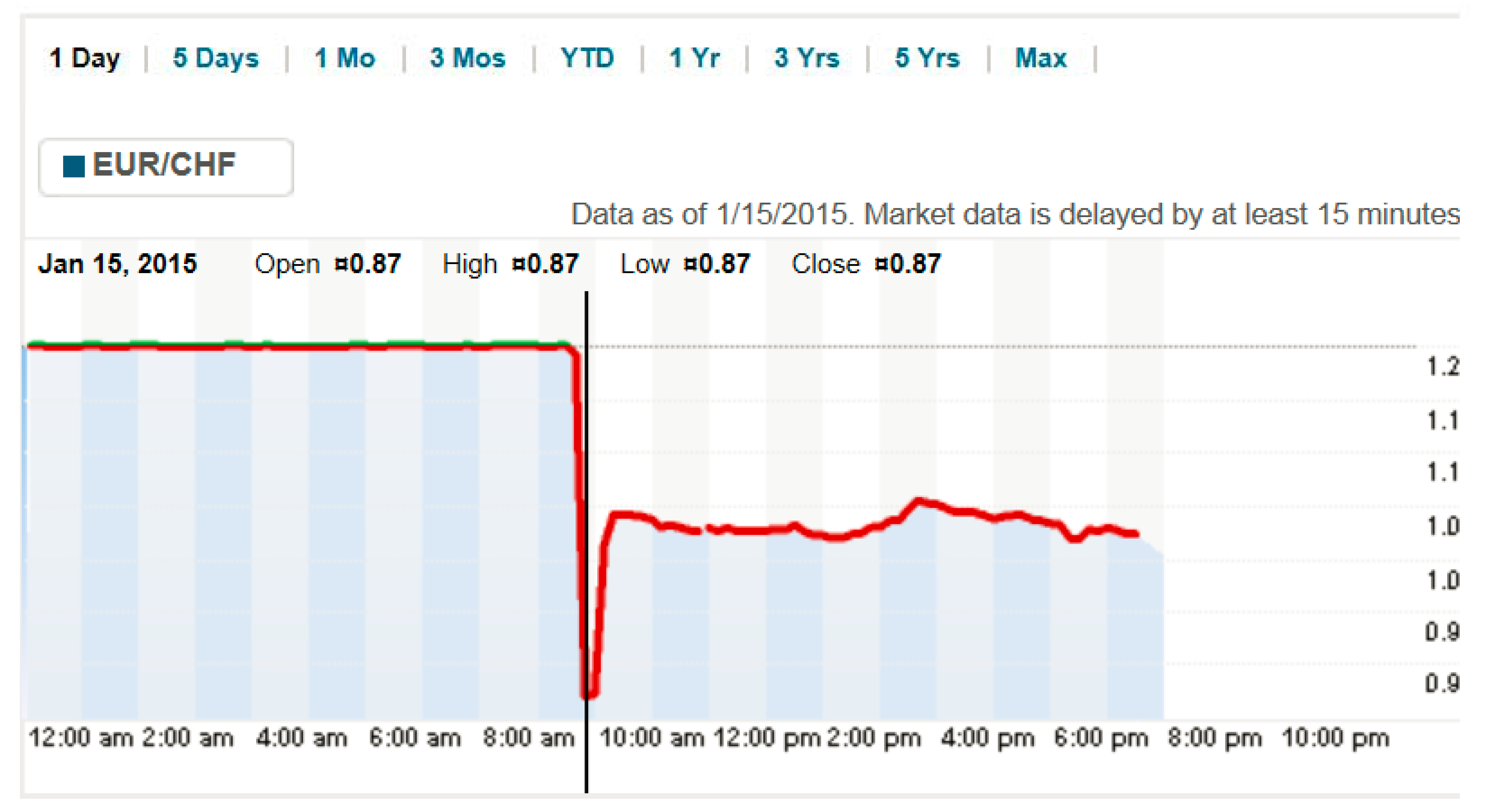
Source: Bloomberg 15 January 2015. Down is an appreciation of the CHF against the EUR.

The expansion in the SNB’s balance sheet as a consequence of foreign exchange intervention is shown in Figure 1. Also shown is the stabilization of the real trade weighted CHF as a consequence of the foreign exchange (euro) intervention.

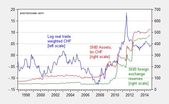
Figure 1: Log real trade weighted value of the Swiss Franc, 2010=0 (blue, left scale, up is a real appreciation of the CHF), and asset side of the SNB balance sheet (red, right scale), and foreign exchange reserves (green, right scale), in billions of CHF. Source: BIS and SNB.

Weisenthal reports speculation that the SNB will focus more on the trade weighted SNB, and perhaps shift intervention to the USD/CHF pair, especially as the path for the ECB’s quantitative/credit easing program is cleared.[1]

Update, 5:50PM Pacific: The appreciation today restores the USD/CHF bilateral exchange rate to that obtaining on 7/14/2014.

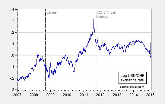
Figure 2: Log USD/CHF exchange rate. Source: FRED and Pacific Exchange Rate Services.

The CHF is about 4% stronger against the USD than it was on 9/7/2011 (the day after the imposition of the cap), while the US CPI has risen about 5% relative to the Swiss CPI since 2011M09. Hence, the real US-Swiss bilateral rate is about the same as it was when the cap was imposed.

Buckle up, it’s going to be a bumpy ride:

Bloomberg on volatility; expect Europe EM balance sheet problems associated with external CHF liabilities.

I Agree with Ed Lazear (and Alan Auerbach)!

If you dynamic score, dynamically score both expenditure and revenue measures.

Professor Lazear writes in a WSJ Op-Ed (ungated version):

Every piece of legislation has economic consequences. Most are small, but some are significant. When the CBO ignores them, it disregards the detrimental effects on economic growth of bad legislation as well as the positive effects on growth of good legislation.

While Professor Lazear argues for dynamic scoring of tax legislation, he also argues for scoring of spending components. This puts both Professors Krugman and Lazear in agreement with Alan Auerbach (UC Berkeley) as well as yours truly. Unfortunately, as Krugman observes I think correctly, the desire to implement dynamic scoring is driven mainly by political objectives (lower taxes overall) rather than a desire to do the economic analysis correctly. Or, — despite the fact that I don’t usually use sports analogies — as succinctly put by Tom Toles: