Menzie David Chinn's Blog, page 34

One Department to Rule Them All

Not my idea! With apologies to JRR Tolkein.

One the Regents candidates nominated by Governor Walker (from Wisconsin Public Radio):

Gov. Scott Walker’s latest appointment to the University of Wisconsin Board of Regents told a state Senate panel on Thursday that the UW should consider eliminating duplicative degree programs on some campuses.

Walker appointed Michael M. Grebe to a seven-year term on the Board of Regents. Grebe’s father, Michael W. Grebe, is the president and CEO of the conservative Bradley Foundation who chaired Walker’s gubernatorial campaigns.

The younger Grebe is an attorney and executive vice president at HUSCO International, a Waukesha-based hydraulics manufacturer. At his Senate confirmation hearing, Grebe said the UW needs to be more efficient, suggesting that could mean eliminating degree programs on some campuses if they’re available on others.

I think this idea has merit of a certain kind. Why should we be granting degrees in economics in multiple campuses of UW? We should just be granting one degree in economics — my vote is for the Madison campus to be it. Also, why degrees in math at different campuses? My vote, UW Madison. Next, chemistry. I think it could profitably be centralized in one campus. My vote – Madison!

Assessing the Rational Agent Response to Elimination of Tenure in Wisconsin State Statute

Thinking about “Exit, Voice and Loyalty” in Wisconsin

The Joint Finance Committee motion to remove tenure from state statute. Winners of the most competitive research awards the University of Wisconsin–Madison provides to its scholars have made a statement, found here.

We are especially concerned about provision 39 of the omnibus motion, which authorizes the Board of Regents to terminate faculty appointments for reasons of “program discontinuance, curtailment, modification, or redirection.” This is a profound departure from current policy, which allows termination of faculty appointments only for just cause after due notice and hearing, or in the event of a fiscal emergency. If passed into law, this provision would greatly weaken any guarantees of tenure provided by the Board of Regents. In essence, state statute would say that tenure at the University of Wisconsin does not mean what it means at every other institution: a guarantee that university administrators cannot arbitrarily dismiss faculty who have earned tenure through research, teaching, and service.

I have seen some individuals (as far as I can tell, typically not involved in knowledge generating sectors of the economy) who asserted that a move to weaken the protections of tenure would eliminate “dead wood”, and reduce costs.

It strikes me that it is useful to consider a rational agent model of individual decision-making, in response to weakening of tenure protections relative to other academic institutions, in assessing the plausibility of such arguments.

First, agents would make the relevant cost-benefit calculations. As costs (from uncertainty) rise, those agents with the highest value of outside options (relative to costs of moving) would move. On average, one would guess that the most accomplished would then tend to move.

Second, the idea of compensating differentials (look at any intro economics textbook) is relevant. If uncertainty is higher, then rational agents — particularly those coming from outside, perhaps as new hires — would tend to demand a higher salary relative to what otherwise would be the case.

Third, the removal of tenure protections could be taken as a signal by state leaders (in the legislature, in the executive) that the contributions by those involved in the academic enterprise are not valued. If leadership at the state level attempts to stifle dissent, then loyalty is reduced, and exit becomes a more attractive option. (Some will recognize this idea from Hirschman.).

So, if one’s objective were to drive out the most academically successful professors, raise cost per unit output of teaching/research (recalling UW brings in billions of dollars of Federal and other grants), and demoralizing the university faculty, then the JFC’s motion is the optimal route.

The entire statement can be found here.

Update: Addition coverage, Herzog/Milwaukee Journal Sentinel, Simmons/Wisconsin State Journal.

A Parsimonious Error Correction Model of Kansas Economic Activity

Or “Kansas macro crash…and burn”

Patrick Marvin argues that Kansas is doing fine, and the tax cuts just need a bit more time to kick in to spur the economy. My reading of the data and estimates suggest otherwise.

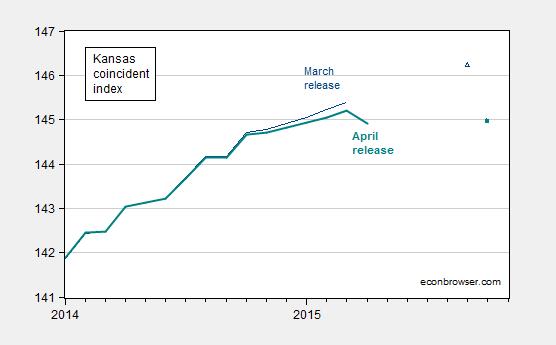
Figure 1: Coincident index for Kansas, March release (dark blue), April release (bold teal). Dark blue triangle (solid teal box) denote corresponding forecasts from March and April releases of leading indices. Source: Philadelphia Fed (coincident), Philadelphia Fed (leading), and author’s calculations.

There has been some debate regarding the pace of economic growth in Kansas over the past four years. In order to compare the outcome with what might be expected, I construct a counterfactual, based upon the historical correlation of Kansas economic activity with US economic activity over the 1979-2015 period. I use as a proxy for economic activity the Philadelphia Fed’s coincident indices, which apply the Stock-Watson approach to extracting a state factor from multiple time series (of possibly differing frequencies).

The log of the coincident series for Kansas and the US do not reject the I(1) null at conventional levels. At the same time, they appear to be cointegrated according to standard test (Johansen, constant, no trend, 3 lags of first differences, at 10% msl).

Hence, I estimate a single-equation error correction model, assuming US economic activity is weakly exogenous for Kansas, over the 1986M01-2010M12. Let ks be the log coincident index for Kansas, and us be the log coincident index for the US. Δ is the first difference operator. The resulting estimates are:

Δwit = –0.001 – 0.0047kst-1 + 0.0049ust-1 + first and second lags of first differences

Adj-R2=0.74, SER = 0.0017, N = 380. Significance at 10% msl denoted by bold face.

Observation 1: This is a pretty high coefficient of variation. Statistically, the m/m growth rate in Kansas economic activity is well explained.

Observation 2: The cointegrating relationship between Kansas output and US is about 1.03.

Observation 3: Estimating the equation over the entire 1990M01-2015M03 does not yield similar coefficients.

I use the equation estimated over 1979-2010 to dynamically forecast out of sample over the 2011M01-2015M03 period, taking as given the ex post realization of the US coincident index. (Technically this is a ex post historical simulation.)

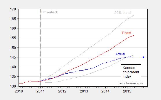
Figure 2: Coincident index for Kansas (blue), ECM forecast (red), and 90% confidence band (gray). Observation for October (blue square) is implied by April leading index. For forecast, see text. Source: Philadelphia Fed (April releases) and author’s calculations.

This outcome suggests that Kansas has been underperforming since 2012M01 relative to a counterfactual based on historical correlations in place over the 1979-2010 period. As of April 2015, actual activity is 7.4% (log terms) below what it should be.

Guest Contribution: “Inflation Expectations Spur Consumption Expenditure”

Today we are fortunate to have a guest contribution by Michael Weber, assistant professor at the University of Chicago’s Booth School of Business. This post is based upon a paper, co-authored with Francesco D’Acunto and Daniel Hoang.

Higher inflation expectations increase households’ propensity to purchase durable goods. This positive association is higher for more educated, working-age, high-income, and urban households. We exploit a natural experiment, the unexpected announcement of a VAT increase in Germany in 2005, to show that the effect of inflation expectations on readiness to spend is causal. Our results imply that monetary and fiscal policies that increase inflation expectations can spur aggregate consumption in the short run.

From the Great Recession to the present day, policy makers around the world have been debating as to which policies may increase aggregate demand and bring the economy back to its steady-state growth path. The major problem is that conventional policies, such as lowering nominal interest rates, are not in the policy toolbox, because rates have hit the zero lower bound (Bernanke, 2010; Blanchard, Dell’Ariccia, Mauro, 2010). Macroeconomic theory suggests that managing inflation expectations may be a useful policy measure: higher inflation expectations would lower the real interest rates in times of fixed nominal rates (Fisher equation), and lower real rates would stimulate consumption (Euler equation).

Surprisingly, there has been no evidence in micro data thus far that these intuitive channels may indeed spur the readiness of households to spend. If anything, the current literature suggests no effect of inflation expectations on readiness to consume (Bachmann, Berg, and Sims, 2015).

Inflation Expectations and Consumption Expenditure: Baseline and Heterogeneity

In a recent paper (D’Acunto, Hoang, and Weber, 2015), we use novel and unique German micro-level data from January 2000 until December 2013. We indeed find that inflation expectations are positively associated with the readiness to spend on durable goods. Figure 1 documents this result in a time series scatter plot. We use the confidential micro data underlying the GfK Consumer Climate MAXX survey. GfK asks a representative sample of 2,000 households every month whether it is a good time to purchase durable goods given the current economic conditions. Higher values correspond to better times. GfK also asks how consumer prices will evolve in the next twelve months compared to the previous twelve months. We create a dummy variable that equals 1 when a household expects inflation to increase. Figure 1 plots the average monthly readiness to purchase durables on the y-axis against the average monthly inflation expectations. Inflation expectations and readiness to spend on durables are strongly positively correlated. Temporarily higher inflation expectations indeed stimulate current consumption spending.

The GfK data also include a rich set of individual characteristics of respondents, including detailed demographics, expectations about household- and economy-wide future economic outlook, and perceptions about the evolution of economic outcomes in the past. In a multinomial logit specification that controls for household-level heterogeneity, we find that households that expect inflation to increase in the following twelve months are 8% more likely to be willing to buy durable goods, compared to households that expect inflation to be stable or decrease in the following twelve months.

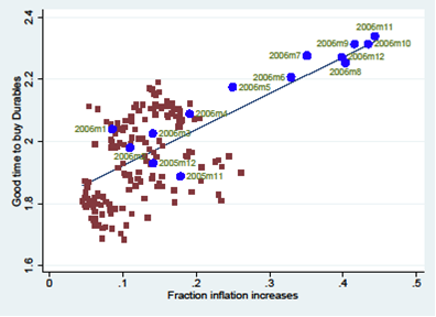
Figure 1: Readiness to Spend on Durables and Inflation Expectations

The richness of the individual characteristics in the GfK data also allows us to study the heterogeneity of the effect of inflation expectations on the readiness to consume across several dimensions. We find that the effect is significantly stronger for the more educated household heads, for higher-income households, for households living in larger cities, and for working-age household heads.

The heterogeneity in the response of households to policy measures emphasizes a challenge for fiscal and monetary policy makers: the intended effects of their policies should be clearly stated, and the types of households that seem less responsive to these measures—that is, lower-income, lower-educated, and retired households, living in rural areas—should be targeted with specific communicative efforts so that the policy measures indeed deliver their full potential.

Inflation Expectations and Consumption Expenditure: A Causal Effect?

Observing detailed household- and economy-wide characteristics helps to control for the heterogeneity across households when estimating our effect. But the analysis thus far does not allow us to claim that the effect of inflation expectations on the readiness to consume is causal. Ideally, we would need a shock to inflation expectations which is exogenous to the characteristics of households, and which only affects a group of treated households. To get close to such an ideal experiment, we exploit a natural experiment. In November 2005, the newly-formed German government unexpectedly announced a three-percentage-point increase in the VAT effective January 2007. The narrative records show that the VAT increase was not legislated for reasons related to future economic conditions, but to consolidate the federal budget. The announcement of the VAT increase was an unexpected shock to German households’ inflation expectations, and should have resulted in higher consumption expenditure as long as nominal interest rates did not increase sufficiently to leave real rates constant, which is exactly what is suggested by the narrative records on the European Central Bank decision-making process.

Of course, German households alone do not allow for a causal test, because all Germans were exposed to the VAT shock. To construct a viable counterfactual for German households, we look at households in other countries of the European Union. We obtained access to the confidential micro-data for three countries (France, Sweden, and the United Kingdom) through national statistical offices and GfK subsidiaries. A concern is whether these households represent a plausible counterfactual for the behavior of German households had the VAT shock not happened. Figure 2 provides evidence that indeed foreign households may represent a viable control group.

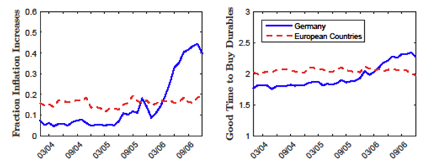
Figure 2 Inflation Expectations and Readiness to Spend on Durables: Germany vs. Foreign

Figure 2 shows that the trends of both average inflation expectations and average readiness to spend on durables were similar for German and foreign households before November 2005, which is 14 months before the start of the VAT increase. We construct a difference-in-differences identification strategy. We compare the outcomes of German households to those of foreign households, both before and after the VAT tax increase shock. To run the analysis at the household level, we match German households with similar foreign households before the announcement of the VAT increase in November 2005. The matching is based on the propensity score to be treated with the shock, estimated with a set of observables that are homogenously elicited across households in various countries through the harmonized questionnaire from the Directorate General for Economic and Financial Affairs. We test formally that, after the matching, German and foreign households are indistinguishable across the matched observables.

In January 2006, that is, twelve months before the announced VAT tax increase, German households are 3.8 percentage points (s.e. 1.5 percentage points) more likely to declare that it is a good time to purchase durable goods after the announcement compared to before, and compared to the matched foreign households. Interestingly, we find that the effect builds up over time in 2006. Figure 3 reports the size of the monthly estimated effect over time.

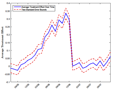
Figure 3: Change in the Readiness to Spend on Durables: German vs. foreign households

The effect increases in magnitude throughout 2006 and peaks at 34 percentage points in November 2006. The average treatment effect drops to zero in January 2007 once VAT actually increases and higher inflation materializes. Interestingly, we do not detect any reversal of the positive effect of the VAT shock on the willingness to purchase durable goods after January 2007. German households behave similarly in their purchasing propensities to matched foreign households not exposed to the shock before the announcement of the VAT increase but also after the actual increase.

Discretionary fiscal policy?

Discretionary fiscal policy is often rejected as a tool for business cycle stabilization. Implementation lags, larger permanent deficits resulting in higher long-term interest rates and distortionary future taxes, or higher marginal propensities to save out of a temporary tax cut (i.e., lower (old) Keynesian multipliers), make it a less desirable policy tool compared to conventional monetary policy. At the same time, a growing literature stresses the use of fiscal policy to stimulate demand in times when conventional monetary policy is less effective. Farhi and Werning (2013) show theoretically that fiscal multipliers are large and above 1 during a liquidity trap. The central mechanism in their paper is that government purchases lead to higher inflation, lower real interest rates, and, therefore, more consumption today. Feldstein (2003) already stressed earlier that discretionary fiscal policy does not have to rely on questionable income effects, but could fully operate through an inter-temporal substitution channel by increasing private incentives to spend: higher inflation expectations lead to more consumer spending today. The use of unconventional fiscal policy can therefore be expansionary and, at the same time, does not lead to higher budget deficits (Farhi, Correira, Nicolini, Teles, 2013).

Our findings offer direct empirical support for those theoretical papers and provide important implications for policy makers, especially for those coordinating the fiscal and monetary policies of countries that are still struggling to exit the Great Recession, such as Italy and Greece (e.g., Handelsblatt, 2015). A series of pre-announced VAT increases and a simultaneous reduction in income tax rates would result in a predictable increase in inflation without inducing additional uncertainty, would increase consumer spending today, and would not lead to higher budget deficits, all while keeping the total tax burden of households the same.

References

Bachmann, R., T. O. Berg, and E. Sims (2015). Inflation Expectations and Readiness to Spend: Cross-sectional Evidence. American Economic Journal: Economic Policy 7 (1), 1-35.

Bernanke, B., 2010. Monetary Policy Objectives and Tools in a Low-inflation Environment. In Speech at a conference on Revisiting Monetary Policy in a Low-Inflation Environment, Federal Reserve Bank of Boston, October, Volume 15.

Blanchard, O., G. Dell’Ariccia, and P. Mauro (2010). Rethinking Macroeconomic Policy. Journal of Money, Credit and Banking 42 (6), 199-215.

D’Acunto, F., D Hoang, and M. Weber. 2015. “Inflation Expectations and Consumption Expenditure.”

Fahri, E., Correira, I., Nicolini, J. P., and P. Teles (2013). Unconventional Fiscal Policy at the Zero Bound. American Economic Review 103(4), 1172-1211.

Fahri, E. and I. Werning (2015). Fiscal Multipliers. Liquidity Traps and Currency Unions. In preparation for Handbook of Macroconomics Volume 2

Feldstein, M. (2003). A Role for Discretionary Fiscal Policy in a Low Interest Rate Environment. In: 2002 Federal Reserve Bank of Kansas City Annual Conference volume, Rethinking Stabilization Policy.

Handelsblatt, 2015. “Das Geld ist nicht da”

This post written by Michael Weber.

Current economic conditions: not as bad as it sounds

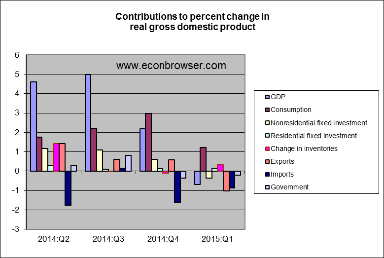
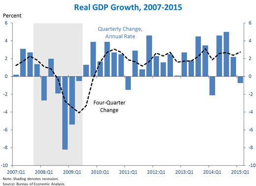
On Friday the Bureau of Economic Analysis released its second estimate of U.S. 2015:Q1 real GDP growth. The BEA now estimates that the economy contracted at a 0.7% annual rate rather than grew 0.2% as originally estimated. The number is discouraging, though I see some silver linings.

The primary factors that brought GDP growth down from the BEA’s original estimate were stronger growth of imports and a smaller inventory build than originally anticipated. Both components can be volatile, and I would not interpret the latter as a sign of fundamental weakness.

The new BEA data also allow us to calculate an alternative estimate of GDP, building the estimate up from income data instead of expenditures. In terms of the underlying concepts, the income-based and expenditure-based calculations should produce the identical number for GDP. But because the data sources are different, in practice the two estimates differ, with the difference officially reported as a “statistical discrepancy.” While the expenditure-based GDP estimate showed a 0.7% decline at an annual rate, the income-based GDP estimate implied 1.4% growth for the first quarter. Moreover, using the statistical method for reconciling and combining the different estimates proposed by Aruoba, Diebold, Nalewaik, Schorfheide, and Song (ADNSS), the best estimate of first-quarter real GDP growth based on the existing data might be about 2%.

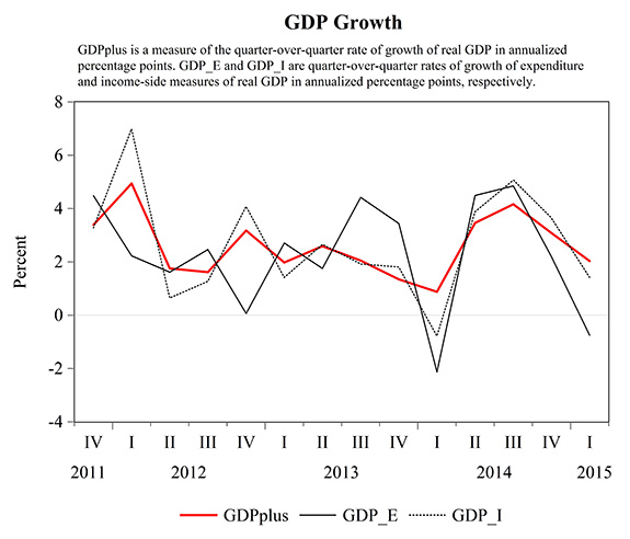
Alternative estimates of real GDP growth at an annual rate. Solid black: expenditure-based estimate reported by BEA. Dotted black: income-based estimate calculated directly from BEA-reported statistical discrepancy and GDP price deflator. Red: estimate calculated using the Aruoba, et al. method. Source: Federal Reserve Bank of Philadelphia.

Another factor contributing to the weak first-quarter GDP number was harsh winter weather. This is becoming a pattern, with the “seasonally adjusted” Q1 estimates coming in consistently below the other three quarters for the last decade. Jason Furman had this comment:

The debate so far over the cause of first-quarter underperformance has tended to treat residual seasonality and weather effects as analytically distinct explanations. However, to the extent that worsening winter weather is part of a long-term trend rather than a random occurrence, changing weather patterns may be related to residual seasonality. A seasonal adjustment algorithm should adjust for effects of normal weather within a particular quarter—and to the extent that global climate change leads to a new “normal” for weather, seasonal adjustments will eventually catch up.

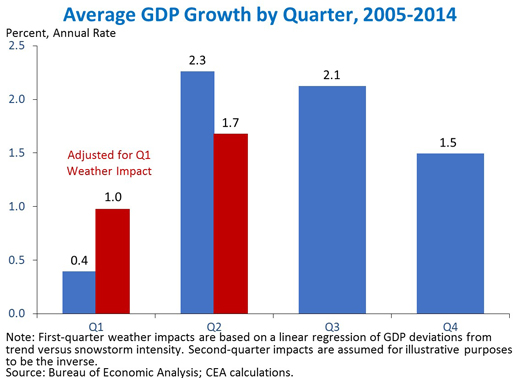
Source: White House Council of Economic Advisers.

But others caution that we shouldn’t simply dismiss the Q1 GDP numbers. Here’s Richard Moody, chief economist at Regions Financial Corp.:

Many analysts seem tempted to simply brush aside the contraction in real GDP in [the first quarter] as a function of transitory factors– harsh winter weather, the port strike– that will have no lasting effect. We caution against treating the first-quarter GDP data so cavalierly, as doing so overlooks the more structural forces that weighed on the economy in [the first quarter]– the ongoing pullbacks in job counts and investment in the energy sector and related industries, still uncertain global growth prospects, and the stronger U.S. dollar.

It’s certainly true that signs of weakness are not just showing up in GDP and are not confined to the first quarter. The latest numbers on industrial production, retail sales, and durable-goods orders all suggest the economy may have hit a soft spot that extended into April.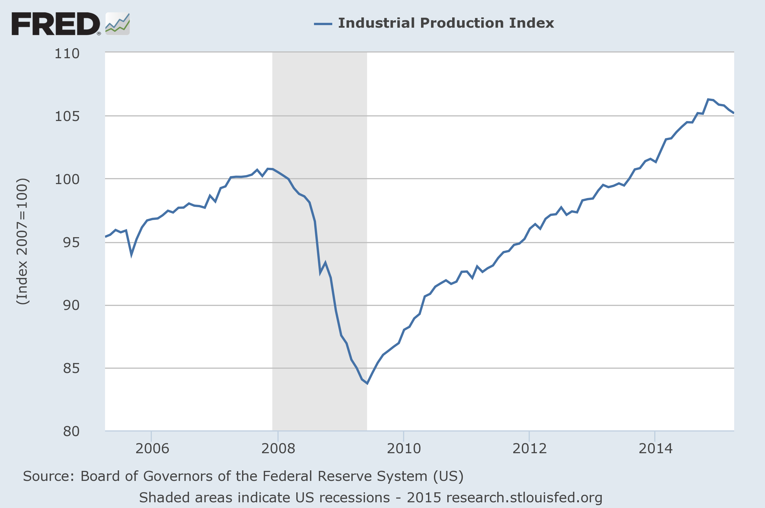

Source: FRED.

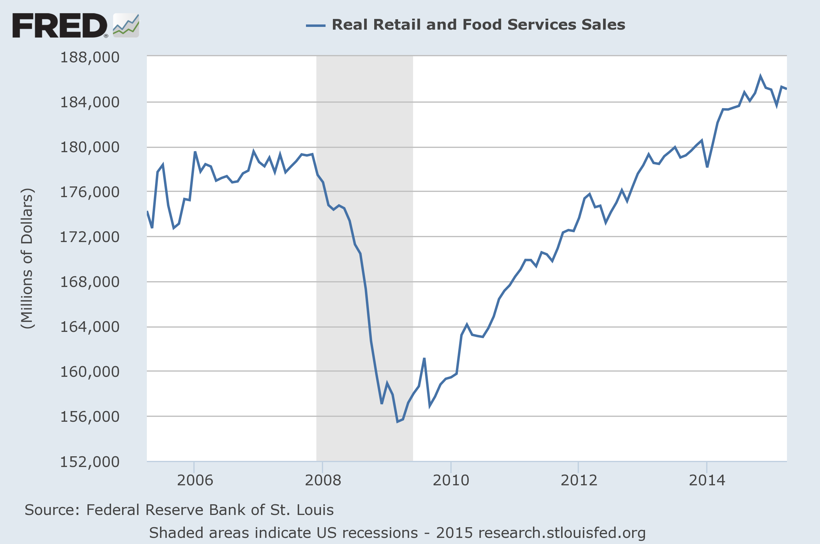
Source: FRED.

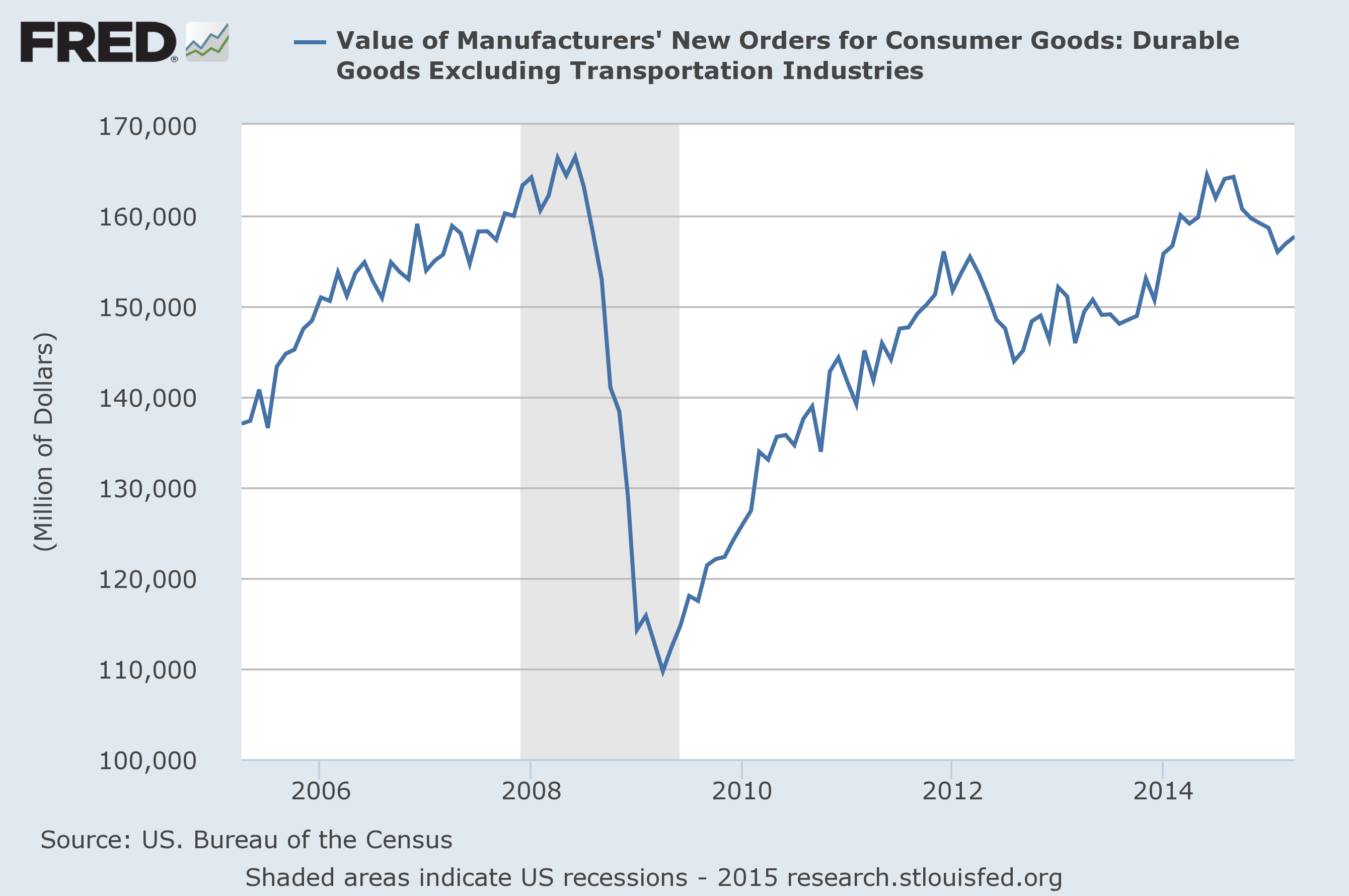
Source: FRED.

But Bill McBride explains why he’s still sanguine about housing:

Total housing starts in April were solid and well above expectations– and at the highest level since 2007…. Note the exceptionally low level of single family starts and completions. The “wide bottom” was what I was forecasting several years ago, and now I expect several years of increasing single family starts and completions.

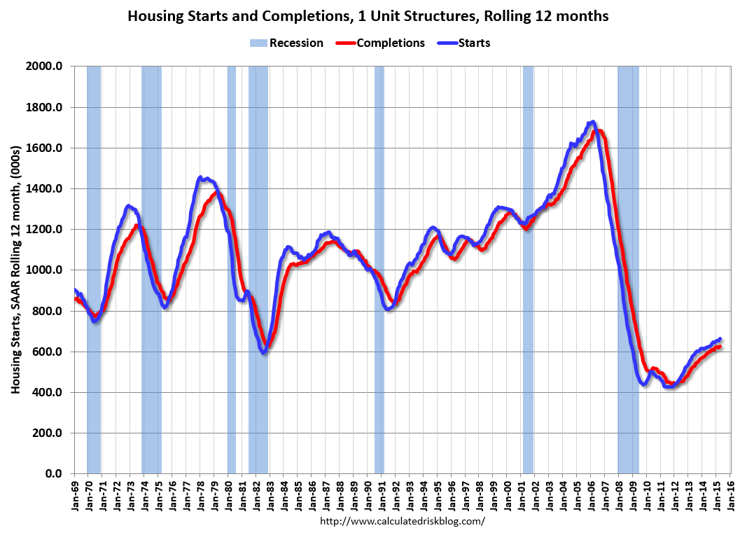
Source: Calculated Risk.

But the key is ongoing gains in employment, which still show solid momentum that should carry the economy forward.

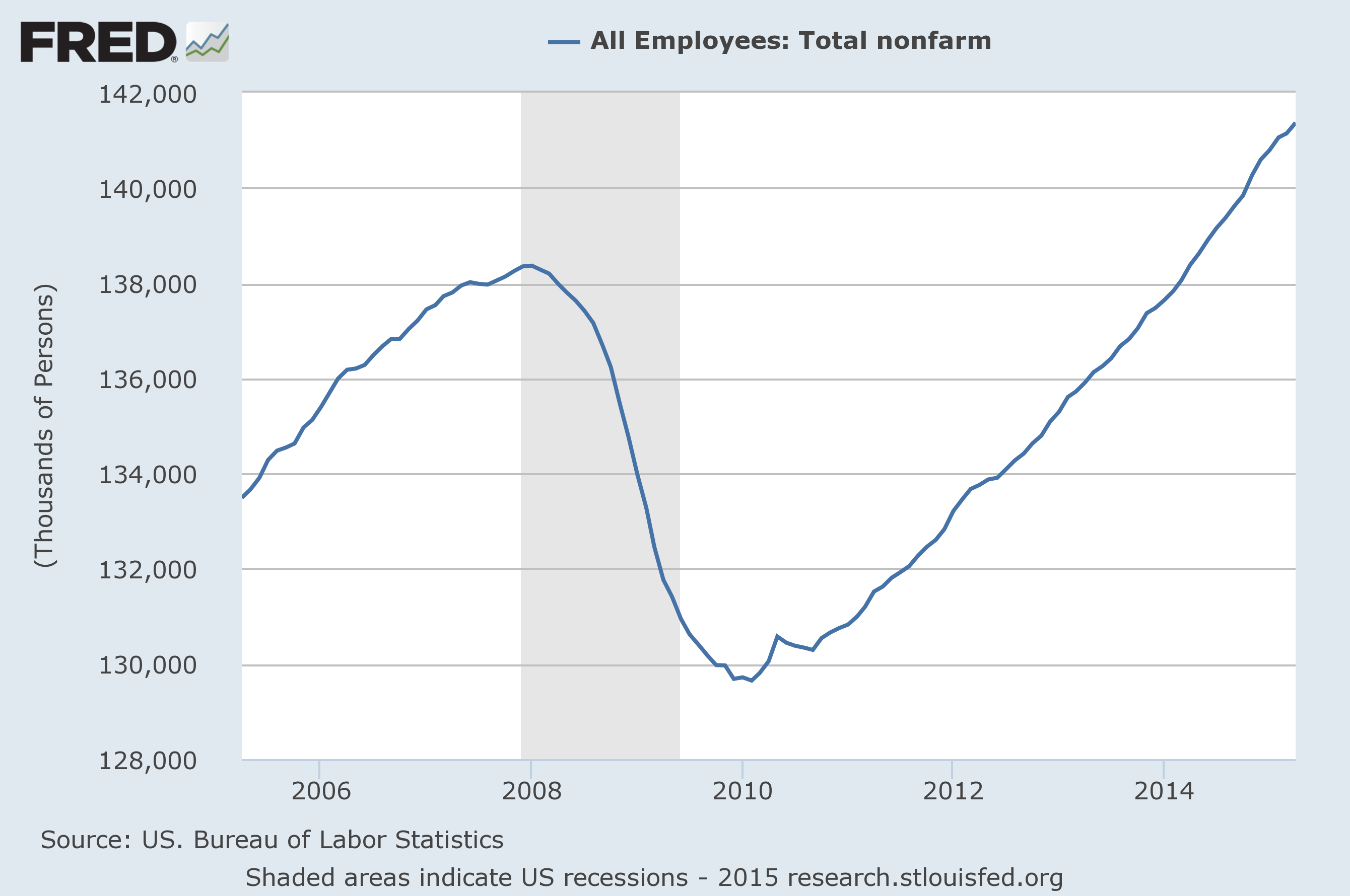
Source: FRED.

Overall, I can’t quarrel with this summary by Council of Economic Advisers Chair Jason Furman:

The first-quarter slowdown was the result of harsh winter weather, tepid foreign demand, and consumers saving the windfall from lower oil prices. The combination of personal consumption and fixed investment, the most stable components of GDP, has grown 3.4 percent over the past four quarters. This solid long-term economic trend complements the robust pace of job growth and unemployment reduction over the last year.

Source: White House Council of Economic Advisers.

Kansas Macro and Fiscal Crash

Economic activity stalls, and the Republicans conclude that higher taxes are necessary for higher tax revenue.

Figure 1 depicts log coincident indices for Minnesota, Wisconsin, California, Kansas, and the US, as compared to 2011M01, when Governors Walker and Brownback took office.

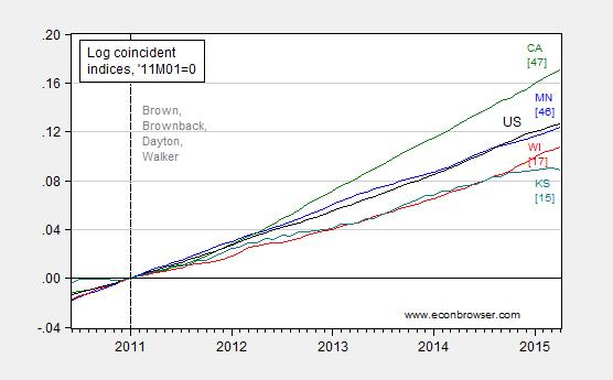
Figure 1: Log coincident indices for Minnesota (blue), Wisconsin (red), California (green), Kansas (teal), and the US (black), normalized to 2011M01=0. ALEC-Laffer Rich States, Poor States, 2014 rankings in brackets. Source: Philadelphia Fed (April release), RSPS 2014, and author’s calculations.

Three month growth in Kansas has flattened (-0.08%, annualized, in logs), and in fact the (preliminary) m/m annualized growth rate for Kansas is -2.4%. This is in sharp contrast to the other states in the graph, including Wisconsin which itself has lagged relative to the US and Minnesota, and lagged relative to what historical correlations up to 2010 would have indicated (and statistically significantly so). In other words, “wow!”.

Figure 2 depicts the March and April releases of the Kansas indices. Notice the recent downward revision. That is, more recent data is not improving the outlook.

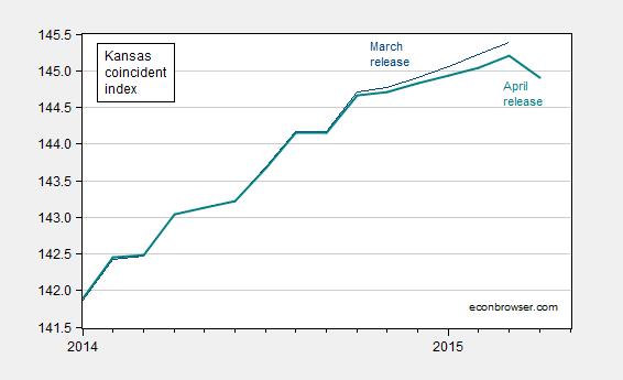
Figure 2: Coincident index for Kansas, March release (dark blue), April release (bold teal). Source: Philadelphia Fed.

The March release of the Philadelphia Fed’s leading indices projected 0.6% growth over the next six months (non-annualized). Given the fact that the leading indices are based on time series models of the coincident, my guess is for a downgrade in the April release (on June 2).

More data on Kansas, from the Kansas City Fed.

On the budget side, the situation has deteriorated as well, going from bad to worse. $400 million gap that is widely cited in the media is actually likely an understatement. As noted by Goossen at Kansas Budget blog, the $400 million presupposes a set of short-term fixes in the form of transfers. Closing the $400 million gap by “…by increasing the state sales tax to 6.65 percent from 6.15 percent and eliminating most income tax deductions” [Foxnews] would leave only $81 million in reserve, when state law requires an end-year balance of about $500 million.

Wisconsin GOP Targets Faculty Tenure

From Greg Neumann/WKOW:

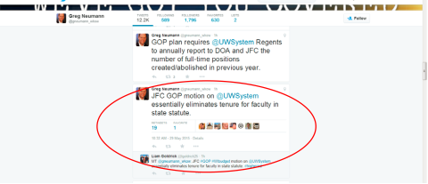
“JFC” is Joint Finance Committee. The text of the motion is here. Stein and Herzog/Journal Sentinel here. The article notes the following contrast: “Minnesota raised taxes with part of the new revenue set aside for higher education.”

“Crony Capitalism”: Wisconsin Edition

RightWisconsin writes:

…crony capitalism is currently wreaking havoc on the conservative Republican brand of free markets and limited government.

The most obvious example of crony capitalism came this weekend with the Wisconsin State Journal’s blockbuster story about another loan gone bad from the Wisconsin Economic Development Corporation (WEDC). The storyline is rather predictable: a politically connected company comes to WEDC and secures a taxpayer-funded loan, then goes belly up fleecing the taxpayers.

The conversion of the Commerce Department into the WEDC was a cornerstone of Governor Walker’s agenda for creating 250,000 new jobs by the end of his first term (actual count according to Quarterly Census of Employment and Wages, 129,131). [1]

Bloomberg has the entire story, which is emblematic of the last four years.

Update: And here is the Governor’s views on government mandated ultrasounds.

Gasoline prices and consumer sentiment

U.S. retail gasoline prices last week averaged over $2.80 a gallon, thirty cents higher than a month ago. The preliminary University of Michigan index of consumer sentiment for May was 88.6, down 7 points from the month before. Are these two developments related?

The consumer sentiment index is plotted in black in the graph below with units on the left scale. The negative of the gasoline price in real terms (deflated using the CPI) is shown in blue, with units on the right scale. I have plotted the negative of gasoline prices to help highlight the negative relation between the two series– when gasoline prices go up (a fall in the blue line), consumer sentiment goes down (a fall in the black line). Consumer sentiment had been improving steadily as gas prices fell (or the blue line rose) last autumn. Since gas prices came back up, sentiment has tumbled.

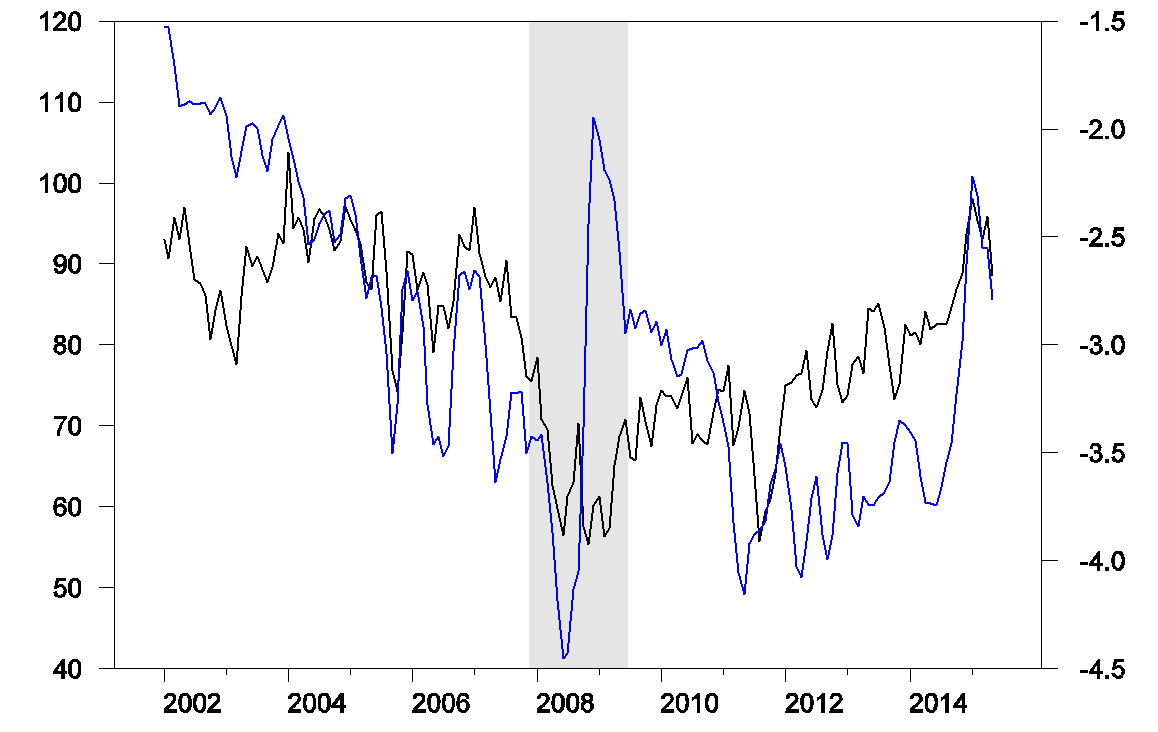
Black: University of Michigan consumer sentiment, 1978:M1-2015:M5 (May 2015 is preliminary estimate, scale is on left). Blue: negative one times the average real U.S. retail price of gasoline, all formulations, in April 2015 dollars per gallon as calculated by deflating by the CPI (May 2015 is preliminary estimate, scale is on right).

One quick way to describe the relation between these series is with a regression of each month’s change in consumer sentiment on that month’s change in the real price of gasoline. Results of that regression are reported below, with t-statistics in parentheses. If the monthly price of gasoline were to jump by $1.00/gallon, the regression would predict about a 5-point decline in consumer sentiment.

Although the coefficient is highly statistically significant, this is a much smaller response than had been found in earlier studies such as Edelstein and Kilian (2007). The relation appears to be significantly weaker in the more recent data than was seen in the older data. For example, if we estimate the regression using only data over 1978:M2-2007:M7 (the sample period used by Edelstein and Kilian), the coefficient is -12.0 instead of -4.9. Based on the data prior to 2008, we would expect about a 12-point drop in consumer sentiment if gasoline prices rose by a dollar.

Referring back to the figure above, we can see what seems to have happened. The first time gasoline prices reached $3.00 a gallon in September 2005 (or $3.50 a gallon in 2015 dollars), consumers appeared to be shocked. When it happened again the following summer, the decline in consumer sentiment was much more muted. And when the threshold was crossed a third time the following year there seems to be barely any response. It was only when prices went on to new highs (to over $4.00/gallon in 2008) that it seems to have again caught consumers’ attention. Nonetheless, when gasoline prices plunged as the recession worsened, it brought little cheer– consumers by then had bigger things to worry about. It is only in the data over the last year that the two series are back to tracking each other as closely as they had seemed to a decade ago.

If we use the full-sample coefficient estimate of -5, the 30 cents/gallon increase since April would have been expected to be associated with a 1.5-point drop in consumer sentiment. Even if we used the coefficient of -12 from the earlier data, we would still have only expected to see a 3.6-point drop in consumer sentiment, only about half of what was actually observed.

My conclusion is that rising gasoline prices surely contributed to the recent decline in consumer sentiment. But I suspect that other factors are more important.

Interest Rate Parity and Exogeneity

One of the enduring puzzles of international finance is the fact that the joint hypothesis of uncovered interest parity and rational expectations is consistently rejected, as evidenced by the coefficient estimates in the Fama regression.

The typical approach is to estimate a regression of the ex post change (in logs) of the exchange rate on the interest differential (this is an approximation).

(1)     Δst 1 = β0 β1 (it – it*) εt 1

A commonplace finding is that estimates of β1 is negative and statistically significantly different from unity, which is the posited value under the null hypothesis. Estimates for five bilateral exchange rates (against the US dollar, 1979-2014Q2) are shown as blue bars in Figure 1.

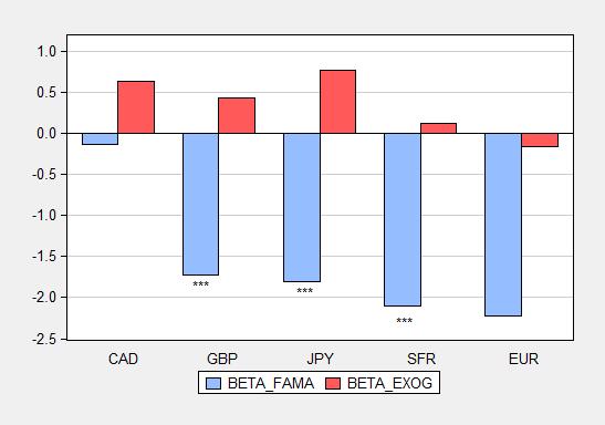
Figure 1: β OLS estimates from equation (1), quarterly data, 1979-2014Q2 period. *** denotes statistically significantly different from unity at 1% level.

One requirement for ordinary least squares (OLS) to yield unbiased estimates is the right hand side variable is uncorrelated with the error term. If the interest rate differential is endogenous (say monetary policy adjusts the interest rate in response to factors impounded in the error term), then estimates could be biased. In Chinn and Meredith (2004), we explicitly model interest rate policy as a function of output and inflation gaps, and inflation and output are a function of exchange rate depreciation; hence in that framework, the right hand side variable is by construction correlated with the error term. A similar approach using a DSGE is undertaken by Chinn and Zhang (2015).

My view is that US monetary policy is less subject to this critique, given the more closed nature of the American economy. One could proceed, using instrumental variables. Another approach is to move the endogenous variable to the left hand side, imposing a unit coefficient.

(2)     Δst 1 – it = β’0 – β1‘ it* ε’t 1

The β1‘ estimates are shown as red bars in Figure 1. Notice that while in a couple cases the β’s appear numerically far away from unity, in no case are the estimates statistically distinguishable from unity.

Is this necessarily the explanation for the biased estimates? It does seem plausible that US interest rates are more exogenous than foreign. Figure 2 plots the 3 month (CD) series used.

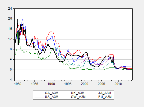
Figure 2: Three month offshore interest rates, end-of-period, %, for US (bold black), Canada (blue), UK (red), Japan (green), Switzerland (chartreuse), and euro (purple).

There might be other explanations, reviewed in for instance Chinn (2006), including more econometric ones (Chinn and Meredith (2005)). An alternative interpretation is that imposing the same β1 on US and foreign interest rates induces correlation between the right hand side variable and the error term.

More on updated results on the Fama regression in this post. Results using survey data as opposed to assuming rational (unbiased) expectations, in this paper.