Menzie David Chinn's Blog, page 31

Possible scenarios for Greece

It’s very clear that two things have to happen from here. First, Greece needs relief from its mountain of debt, and second, the country needs to find a way to become more competitive economically.

The traditional way these goals would be achieved is first, creditors would accept substantial haircuts and restructuring of the outstanding debt, and second, a big currency depreciation would give Greek exports a competitive international advantage to get the economy growing again without new borrowing.

The main complication preventing these steps in the current situation is Greece’s participation in the euro system. On the first issue, this meant that European governments, banks and the ECB extended substantial loans on the (mis)understanding that Greece’s membership in the European union meant default was impossible. On the second issue, devaluation would seem not to be an option because Greece does not have control over the value of its currency.

But the reality that everyone needs to recognize is that, one way or another, both changes are eventually going to happen. It’s just a question of when and how.

That Greece’s creditors are going to have to accept substantial restructuring of the sums they receive is simply an unavoidable consequence of the fact that, through a combination of a lack of tangible economic resources and the reality of Greek politics, Greece isn’t able to make the annual interest payments on its current load of debt. This reality has been quite evident for some time, though up to now Europe kept valiantly kicking this can down the road.

Gross debt of the Greek government as percent of GDP, 1980-2013. Data source: IMF World Economic Outlook Database.

And if we do not get a real depreciation in the form of a change in the nominal exchange rate, the same goal can be achieved through a big drop in Greek wages and prices. The trouble is, this normally doesn’t happen unless there is a huge amount of unemployment. For example, it took the Great Depression of 1929-33 in the United States to bring prices and wages here down by a third. The New York Times has some eye-opening graphs demonstrating that the downturn in Greece has already become worse than what the U.S. saw in the Great Depression of the 1930s.

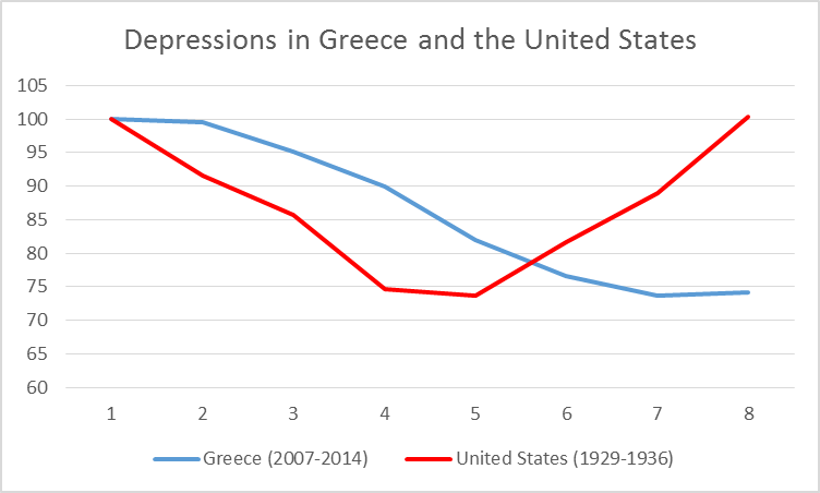
Red: U.S. real GDP, 1929-1936, as a percent of 1929, plotted as function of number of years since 1929 (data source: FRED). Blue: Greece real GDP, 2007-2014, as a percent of 2007, plotted as a function of number of years since 2007 (data source: IMF World Economic Outlook Database).

But it would have been so much easier if, rather than ask workers and pensioners to accept a 20% cut, Greece instead experienced a 60% increase in prices of imported goods with nominal wages and pensions unchanged. In the latter case, it would be clear to everyone that the painful adjustments were an unavoidable consequence of international developments and the country’s current circumstances, rather than a deliberate decision by some perceived political or economic adversary. Greece could become more competitive without having to go through a depression to get there.

Is there any better way to do this without leaving the euro? Here’s one idea that may sound a little crazy, but perhaps no less crazy than some of the wishful thinking that’s been calling the shots so far. Suppose the Greek government were to declare, we simply do not have the euros to make the payments we’ve promised to government workers, pensioners and suppliers of goods and services to the government. So we will make those payments 60% with euros and 40% with newly created Government Value Certificates. What are these certificates good for? Well, one thing you can do is pay up to 20% of any tax obligations you have with them, at par (one certificate discharges one euro in tax obligations), this year, or any time in the future. Greece might also consider a law specifying that a private firm could fulfill its legal obligations to employees by paying up to 20% of the euros owed with certificates.

Such certificates would have a direct market value. If you wanted, you could sell any certificates you have or buy any certificates you want from somebody else. The certificates would trade on the private market at a significant discount from par, based on factors such as how many new certificates people expect the government to issue next year and how useful they’re expected to be for paying future taxes. The size of the discount would determine how much of a de facto devaluation the program could achieve. In effect, this would amount to introducing a parallel currency.

Maybe you like that proposal, or maybe you don’t. But either way, some combination of debt forgiveness and real depreciation is going to occur, whether we like it or not.

And the sooner it happens, the better it will be for everyone.

The Information Content of the ALEC-Laffer-Moore-Williams Economic Outlook Ranking

An Econometric Assessment of the World according to the American Legislative Exchange Council (ALEC)

For eight years, the American Legislative Exchange Council has been producing a ranking that purports to measure the competitiveness of individual states. From ALEC, Rich States, Poor States, 2015:

The Economic Outlook Ranking is a forecast based on a state’s current standing in 15 state policy variables. Each of these factors is influenced directly by state lawmakers through the legislative process. Generally speaking, states that spend less—especially on income transfer programs, and states that tax less—particularly on productive activities such as working or investing—experience higher growth rates than states that tax and spend more.

Hence I think it is reasonable to ask whether the ALEC-Laffer-Moore-Williams “economic outlook” ranking (hereafter “ALEC ranking”) actually has any predictive power, above and beyond other demographic and geographic indicators. This analysis follows up on a more ad hoc analysis in this post, and confirms conclusions arrived at in Fisher w/LeRoy and Mattera (2012). In addition, this analysis serves as a rejoinder to ALEC’s rebuttal asserting that critiques did not incorporate sufficient controls and allow for differing time horizons, to wit:

Moreover, rigorous statistical methods show that a higher economic outlook ranking in Rich States, Poor States does indeed correlate with a stronger state economy.

H/t Michael Hiltzik, who has done a tremendous job tracking the ALEC ranking. Let’s examine the available data.

Figure 1 depicts the one year growth in real Gross State Product and the ALEC ranking, lagged one year, for growth over the 2008-2014 period. Should the ALEC thesis be correct, one should see a negative sloped relationship.

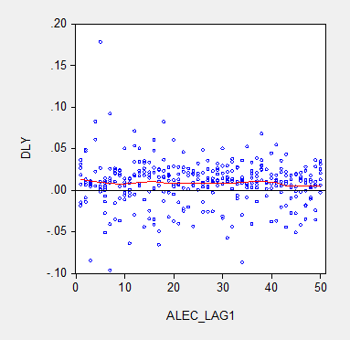
Figure 1: Real Gross State Product growth (log first difference) and lagged ALEC ranking for Economic Outlook. Nearest neighbor fit line (red), window = 0.3. Source: BEA and ALEC, Rich States, Poor States, 2015, and author’s calculations.

There is no obvious correlation between annual growth rates and the ALEC rankings. Note that lagging the ranking so that, for instance, the growth rate between 2013 and 2014 is related to the ALEC ranking in 2012 (instead of 2013) does not change the results much. (The ALEC 2013 ranking pertains to data reported in 2012, as far as I can tell). This outcome is unsurprising because the ALEC rankings are highly persistent. If one estimates a panel autoregressive model for the ALEC rankings, the AR coefficient is 0.95, and the adjusted R2 is 0.90.

Defenders of the ALEC rankings have argued that the rankings are aimed at predicting growth at a longer time horizon than annual. Given that the perspective of the RSPS methodology is supply-side, this argument is prima facie sensible. In order to accommodate that argument, I display in Figure 2 the data for three year (nonoverlapping) horizons (for 2014, and 2011).

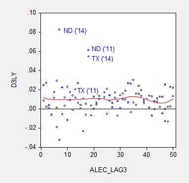
Figure 2: Nonoverlapping average three year real Gross State Product growth (log difference) and three year lagged ALEC ranking for Economic Outlook. Nearest neighbor fit line (red), window = 0.3. Source: BEA and ALEC, Rich States, Poor States, 2015, and author’s calculations.

Figure 3 provides analogous information, at the six year horizon (the maximum possible given the span of ALEC rankings).

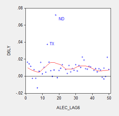
Figure 3: Nonoverlapping average six year real Gross State Product growth (log difference) and six year lagged ALEC ranking for Economic Outlook. Nearest neighbor fit line (red), window = 0.3. Source: BEA and ALEC, Rich States, Poor States, 2015, and author’s calculations.

The nonparametric fitted lines indicate a slightly negative slope overall, suggesting some content to the argument that lower ranked states grow slower. In both Figures 2 and 3, North Dakota and Texas constitute outliers along the y-dimension. In order to discern how much these two observations drive the results, I omit them and replot in Figure 4.

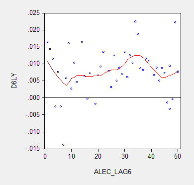
Figure 4: Nonoverlapping average six year real Gross State Product growth (log difference) and six year lagged ALEC ranking for Economic Outlook, excluding North Dakota and Texas. Nearest neighbor fit line (red), window = 0.3. Source: BEA and ALEC, Rich States, Poor States, 2015, and author’s calculations.

No obvious pattern emerges from this last plot. In order to move beyond simple graphics, I now implement a series of regressions. First to a simple examination of the a bivariate relationship, encompassing the lower 48 states, one obtains at the annual frequency:

Δyi,t = -0.00003ALECi,t-1

Adj-R2 = -0.00, SER = 0.027, N=288. bold indicates significance at 10% msl, using heteroscedasticity and serial correlation corrected standard errors.

(I use the lower 48 as I do not have demographic and geographic data for the Alaska and Hawaii.)

Essentially, there is no explanatory power for the ALEC-Laffer indices in terms of year on year GSP real growth. Allowing for individual state-fixed effects, one obtains:

Δyi,t = 0.0004ALECi,t-1

Adj-R2 = -0.00, SER = 0.027, N=288. bold indicates significance at 11% msl, using heteroscedasticity and serial correlation corrected standard errors.

The coefficient is positive, indicating that lower ranked states, and hence states that have a less business friendly environment according the ALEC criterion, exhibit higher economic growth. The coefficient is borderline statistically significant. I would say that the use of state-level fixed effects is a fairly blunt way to account for state-specific factors. A better approach controls for state factors that economic theory suggests might be important for growth, such as geographic and demographic factors. Here we include log population density (LDENSITY, to account for urbanization), dryness (measured as inverse, WET), mildness of weather (MILD) and proximity to navigable waterways (DISTANCE); these four variables are defined such that positive coefficients are expected. These variables are time-invariant; hence one cannot estimate a fixed effects regression incorporating these variables. I also include log real price of oil (LRPOIL) to control for oil producing states, allowing the coefficient to vary across states.

Δyi,t = 0.0002ALECi,t-1-0.01LDENSITYi + 0.019WETi + 0.001MILDi + 0.0001DISTANCEi + LRPOILi,t

Adj-R2 = 0.36, SER = 0.021, N= 288. bold indicates significance at 10% msl, using heteroscedasticity and serial correlation corrected standard errors.

The ALEC ranking has no statistical significance, while a drier and more mild climate is associated with faster growth, with statistical significance. Proximity to navigable water is also a positive factor.

What if we estimate a comparable regression, looking at 6 year growth rates (but omitting oil prices which are the same for all states)? Then one obtains:

Δyi,t = -0.018 -0.0001ALECi,t-6 +0.001LDENSITYi – 0.0007WETi – 0.0003MILDi -0.00001DISTANCEi

Adj-R2 = -0.02, SER = 0.007, N= 48. bold indicates significance at 10% msl, using heteroscedasticity and serial correlation corrected standard errors.

Notice that the ALEC coefficient is not statistically significant. Thus far, the one case it has shown up as borderline significant, it goes the opposite of the ALEC-Laffer-Moore-Williams thesis.

Finally,Professor Ed (“no recession”) Lazear recently asserted that states with fast growing employment have low tax rates and right-to-work laws. He also argues that one needs to incorporate the depth of the drop in employment in 2008-09, in order to explain the growth in employment (so, a sort of version of the bounceback thesis he forwarded in the Economic Report of the President, 2009). I can’t find the working paper that provides the basis for his assertion, but I can estimate a comparable regression. In order to make the proposition testable, I examine 5 year growth rates in output, and refer to the ALEC rankings in 2009. I add the change in output from 2008 to 2009 (so TROUGHDEPTH takes on a value of -0.05 for observation i if output dropped 5% going into 2009).

Δyi,t = 0.065 -0.0010ALECi,t-5 +0.0046LDENSITYi + 0.0042WETi – 0.0014MILDi +0.00005DISTANCEi – 0.3413TROUGHDEPTHi

Adj-R2 = -0.04, SER = 0.037, N= 48. bold indicates significance at 10% msl, using heteroscedasticity corrected standard errors.

The ALEC variable does not exhibit statistical significance (nor does the depth of the drop – and it has the wrong sign). Omitting ND and TX would not change this basic results.

Bottom line: The ALEC ranking, which purports to measure business-friendly policies, is not correlated with real GSP growth, either short term or medium term. This is true if one controls for additional variables.

I don’t think this necessarily means that policies such as right to work, or tax rates, and so forth do not have an impact on growth. For instance, Kolko, Neumark, and Cuellar Mejia, J.Reg.Stud. (2013) conclude that what’s important is “less spending on welfare and transfer payments; and more uniform and simpler corporate tax

structures.” Hence, the ALEC economic outlook ranking is, in my assessment, a manifestation of faith based economics.

Note: Thanks to Professor Neumark, who kindly provided the data set used in his J.Reg.Stud. paper for use by my students in my PA819 statistics course (all students had to use his data set to analyze whether business conditions as measured by various indices (but not the ALEC ranking) influenced state level growth). The demographic and regional variables are drawn from that data set.

China: The Stock Market Meltdown Continues

The stock market continued to decline today, despite vigorous efforts by the authorities. That being said, perspective is required.

The NYT has some good coverage on ongoing stock market developments [1] [2], and why they have occurred.[3] Figure 1 places the current bust in context:

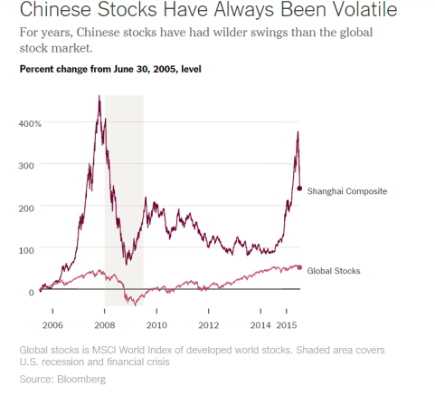
Source: The Upshot/NYT.

Briefly put, there are few alternatives for saving in China. The formal banking system provides negative returns (low deposit yields, lower than inflation typically). Housing is no longer returning positive capital gains — partly as a consequence of deliberate policy actions to moderate a perceived housing bubble. So, what’s left (given you can’t easily save in overseas assets)? Equities. We have a typical boom-bust phenomenon, amplified by underdeveloped financial markets, opacity in valuations, and uncertainty regarding the government’s intentions (and will-power).

But (as befits a macroeconomist), I still think the big picture is the trajectory of the real economy. And here, I think it’s just a matter of how “cool” it becomes. For those who want to see a whole plethora of indicators, go to World Economics’ China Growth Tracker page for July. Quick plots of other data is here at TradingEconomics. People can do their own version of the Rorschak test…

For links to more in-depth analyses of the economic outlook (from the World Bank), and the need for further financial reform, see this post. For discussion of longer term reform needs, see here.

Some Recent Research on Exchange Rates

Here is some interesting work I’ve seen recently in Paris and Cambridge, MA.

First up, the Banque de France and Sciences Po organized a workshop on Recent Developments in Exchange Rate Economics

Here’s the program (links may go to older versions of the papers, and some presentations haven’t quite made it to paper form):

Quality, Trade and Exchange Rate Pass-Through

Natalie Chen (University of Warwick)

Luciana Juvenal (International Monetary Fund)

Discussant: Philippe Martin (Sciences Po)

Invoicing Currency, Firm Size and Hedging

Isabelle Mejean (Ecole Polytechnique)

Julien Martin (Université du Québec)

Discussant: Walter Steingress (Banque de France)

The Dynamics of the Trade Balance and the Real Exchange Rate: The J Curve and Trade Costs?

George Alessandria (Rochester University)

Horag Choi (Monash University)

Discussant: Francesco Pappada (Banque de France)

The Distributional Consequences of Large Devaluations

Javier Cravino (University of Michigan)

Andrei Levchenko (University of Michigan)

Discussant: Daniele Siena (Banque de France)

Revisiting the Fama Puzzle: An Unexpected Journey

Menzie Chinn (University of Wisconsin)

Matthieu Bussiere (Banque de France)

Laurent Ferrara (Banque de France)

Jonas Heipertz (Paris School of Economics)

Discussant: Agnès Bénassy-Quéré (Paris school of economics)

Real Exchange Rates and Commodity Prices

Juan Pablo Nicolini (Federal Reserve Bank of Minneapolis)

Joao Luiz Ayres Queiroz da Silva (University of Minnesota)

Discussant: Julia Schmidt (Banque de France)

Second, yesterday, at the International Finance and Macroeconomics program of the NBER Summer Institute, there were two papers on exchange rates:

If the Fed Sneezes, Who Catches a Cold?

Luca Dedola, European Central Bank

Livio Stracca, European Central Bank

Discussant: Victoria Vanasco, Stanford University

Can Foreign Exchange Intervention Stem Exchange Rate Pressures from Global Capital Flow Shocks?

Olivier J. Blanchard, International Monetary Fund and NBER

Irineu E. de Carvalho Filho, International Monetary Fund

Gustavo Adler, International Monetary Fund

On the Fama Puzzle, I have some other recent work here (with Yi Zhang) and here (with Saad Quayyum).

Ongoing Developments in China

While eyes are on developments in Greece (and rightly so), I thought it would be useful to spend a moment on the uncertainty regarding the Chinese economy’s course (not that I’m the first to point out).

The wild gyrations in the Chinese stock market are displayed in Figure 1; the stock market has doubled over the past year.

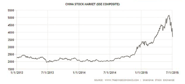
Figure 1: Shanghai Stock Exchange. Source: Tradingeconomics.com

The plunge has spurred a flurry of large interventions by the government, with the government coordinating a fund to buy blue chip stocks, a halt to IPOs, and the move for the PBOC and one arm of the country’s sovereign wealth fund to backstop the stock market by lending to brokerage firms (see Bradsher, Buckley/NYT). This activity follows a series of measures implemented over the past few months.

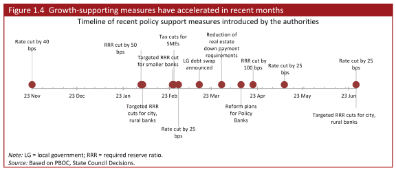
Source: World Bank, China Economic Outlook June 2015 (July 3 update).

The anxiety over the stock market is heightened by the fact that output growth, measured in various ways, is decelerating. A shock to household wealth will surely put a damper on consumption; and a hit to confidence in the government’s economic management cannot help either.

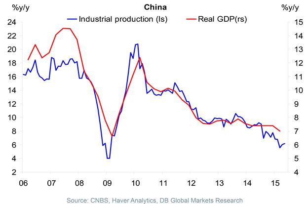
Figure 2: Output measures for China. Source: Torsten Slok/Deutsche Bank (July 2015) [not online].

Some additional current statistics are reported in the World Bank, China Economic Outlook June 2015 (July 3 update). (The current version omits a section on longer term issues regarding the financial system; see here).

Finally, some context. Figure 3 presents the dollar increments to world GDP (in PPP terms, i.e., billions of current international dollars) for 2011-2016. Figure 4 presents the same, except expressed in contributions to world GDP growth.

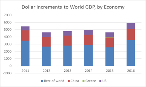
Figure 3: Dollar contributions to world GDP increase, in billions of current international dollars, from US (blue), China (red), Greece (green) and Rest-of-world (purple). 2015 and 2016 observations are IMF estimates from May. Source: IMF, World Economic Outlook May 2015 database, and author’s calculations.

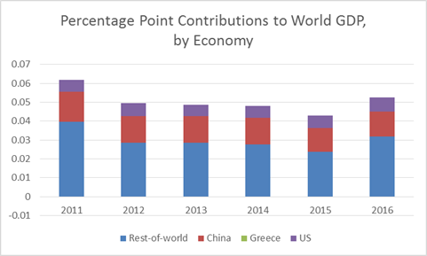
Figure 4: Percentage point contributions to world GDP growth in PPP terms, in decimal form, from US (blue), China (red), Greece (green) and Rest-of-world (purple). 2015 and 2016 observations are IMF estimates from May. Source: IMF, World Economic Outlook May 2015 database, and author’s calculations.

Greece does not show up in either graph; of course, that doesn’t foreclose the possibility that the outcome of the Greek crisis will have outsized financial repercussions.

Latest reports on the Chinese markets as of 9pm Pacific, [1]

We Don’t Need No Stinkin’ Open Records Laws (in Wisconsin)

I guess William Cronon won’t have to worry any more about having his emails scoured by the Wisconsin GOP. From the Wisconsin State Journal:

Legislative Republicans on Thursday passed sweeping changes to the state’s open records law that would dramatically curtail the kind of information available to the public about the work that public officials do.

The proposal blocks the public from reviewing nearly all records created by lawmakers, state and local officials or their aides, including electronic communications and the drafting files of legislation. The language was included in the final version of the state’s 2015-17 budget, which passed the Legislature’s budget committee on a party-line vote late Thursday. The budget bill next goes to the full Assembly and Senate.

From Milwaukee Journal Sentinel:

The Legislature’s Joint Finance Committee tucked the changes to the open records law into the version of the state budget proposal it passed Thursday night. The changes are sweeping, essentially allowing public officials to keep secret records that reveal how they do their jobs.

Like removing tenure from the state charter, this measure seems to have little to do with fiscal issues…If you are wondering who might have pushed this legislation, you can look back to this episode. (Or it could be the WEDC fiasco.)

Happy Fourth of July!

The International Aspects of the Employment Release

The headline number for nonfarm payroll employment was decent [1], and although there are worrisome aspects, I think the key take-away is the fact that manufacturing employment is slowing much more than overall. To the extent that manufactured goods proxies for tradables, I think caution is in order with respect to monetary tightening. And yet, I read headlines reporting that the “Fed is on track to raise rates…”[Sparshott/RTE WSJ].

My argument for deferring monetary tightening follows this sequence.



The dollar’s surge coincides with manufacturing employment slowdown.

The manufacturing slowdown is even more evident in other measures.

The dollar’s movements seems well explained by monetary policy.

Figure 1 illustrates the remarkable surge in the real value of the dollar against a broad basket of currencies — an approximate measure of competitiveness in a macro sense.

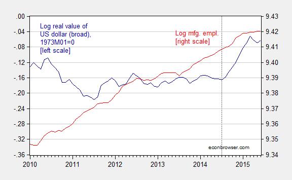
Figure 1: Log real trade weighted value of dollar (broad, 1973M01=0) (dark blue, left scale) and log manufacturing employment, seasonally adjusted (red, right scale). Dashed line at 2014M07. Source: Federal Reserve and BLS.

The manufacturing slowdown is marked in other aspects, as shown in Figure 2.

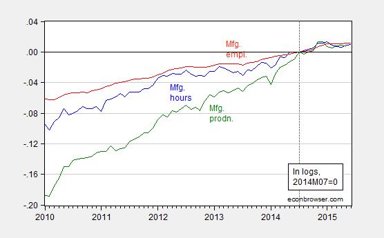
Figure 2: Log aggregate manufacturing hours (blue), log manufacturing employment (red), and log manufacturing production (green), all normalized to 2014M07=0. Dashed line at 2014M07. Source: BLS, Federal Reserve, and author’s calculations.

There is always the temptation to say that exchange rates move in ways mysterious (heck, I’ve contributed to that literature). But I think there is a strong case to be made — stronger than usual — that monetary policy has been driving the dollar’s value. Now, this point can’t be verified by reference to interest differentials, given the zero lower bound. But shadow rates, which summarize anticipations of future rates, do tell a tale, as shown in Figure 3.

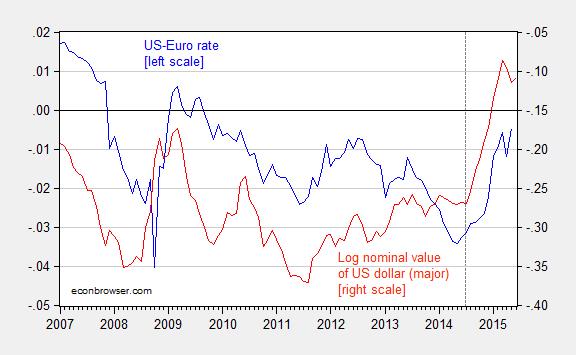
Figure 3: Shadow Fed-ECB interest differential (blue, left scale), and log trade weighted nominal value of US dollar (major) (red, right scale). Source: Xia and Wu, Federal Reserve Board, and author’s calculations.

The correlation is consistent with the view that the extremely rapid rise in the dollar’s value was due to perceptions of rising Fed rates against a backdrop of declining ECB rates. So, if there is anything that is likely to suppress further dollar appreciation, it would be signalling from FOMC members of a slow pace of rate rises, contra what the is being reported Hilsentrath/RTE WSJ.

In the absence of such measures, current forecasts are for more dollar appreciation (For instance, as of today, Deutsche Bank forecasts dollar – euro parity be year’s end). As I noted earlier, another year of appreciation would not be surprising, given historical precedents.

More on the employment release, from [Calculated Risk], [Baker/CEPR], and [Timiraos/WSJ RTE].

Guest Contribution: “Macroeconomic Effects of High-Frequency Uncertainty Shocks”

Today, we are fortunate to have a guest contribution written by Laurent Ferrara (Banque de France and University Paris Ouest Nanterre La Défense) and Pierre Guérin (Bank of Canada). The views expressed here are those of the authors and do not necessarily represent those of the Banque de France or of the Bank of Canada.

Macroeconomic and financial uncertainty is often considered as one of the key drivers of the collapse in global economic activity in 2008-2009 as well as one of the factors hampering the ensuing economic recovery (see, e.g., Stock and Watson (2012)). While it has long been acknowledged that uncertainty has an adverse impact on economic activity (Bernanke (1983)), it is only recently that the interest in measuring uncertainty and its effects on economic activity has flourished (see, e.g., the literature review in Bloom (2014)).

A key issue relates to the measurement of uncertainty. A first solution is to measure uncertainty from news-based metrics. For example, this can be done by counting the number of newspaper articles that contain words pertaining to specific categories, for example, “economy”, “uncertainty” and “legislation”. This is the approach followed by Baker et al. (2013) to estimate daily uncertainty in the U.S. Another solution is to estimate uncertainty from the degree to which economic activity is predictable. This can be achieved by calculating the dispersion in survey forecasts or from the unpredictable component of a parametric model (see, e.g., Jurado et al. (2015) or Rossi and Sekhposyan (2015)). Moreover, uncertainty is also often proxied with a measure of financial market volatility such as the VIX (a measure of the implied volatility of the S&P500).

Despite a large number of uncertainty measures available in the literature, there is a fairly general consensus on the macroeconomic effects of uncertainty, in that uncertainty shocks are typically associated with a broad-based decline in economic activity. In particular, private investment is often estimated to exhibit a strong adverse reaction to uncertainty shocks. However, an interesting recent contribution can be found in the recent IMF’s World Economic Outlook chapter on investment that suggests that, since the onset of the Great Recession, the predominant factor holding back investment is the overall weakness in economic activity (the so-called accelerator effect) while financial constraints and policy uncertainty have a lower explanatory power (see also this previous Econbrowser post).

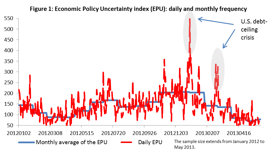
In a recent paper, we evaluate the effects of uncertainty shocks on the U.S. macroeconomic environment. In particular, we concentrate our analysis on the effects of high-frequency (i.e., daily or weekly) uncertainty shocks on low-frequency (i.e., monthly or quarterly) variables. In fact, it is natural to think that there could be insights to gain from the use of high-frequency data in that daily uncertainty measures are often characterized by temporary spikes that are not necessarily reflected in lower-frequency measures of uncertainty (see Figure 1). As a result, aggregating high-frequency uncertainty measures at a lower frequency could lead to a loss in information that may be detrimental for statistical inference. Likewise, if economic agents make their decisions at a high-frequency unit (say weekly frequency) but that the econometric model is estimated at a lower frequency (say monthly or quarterly), this could well lead to erroneous statistical analysis (see, e.g., Foroni and Marcellino (2014)). In the econometric jargon, this is dubbed as a temporal aggregation bias.

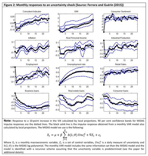
In our empirical analysis, we deal with the mismatch of data frequency between the U.S. monthly macroeconomic variables and the daily uncertainty measures we use (VIX and EPU) by estimating a mixed-data sampling (MIDAS) model that allows us to avoid aggregating the high-frequency data before estimating the models. A number of salient facts emerge from our empirical analysis:



The variables that respond the most to uncertainty shocks are labor market and credit variables (Figure 2). Other macroeconomic variables such as industrial production and survey data (e.g., ISM), also respond negatively to an uncertainty shock, but the responses are rather short-lived.

There is no evidence for a substantial temporal aggregation bias in that responses from mixed-frequency data models typically line up well with those obtained from single-frequency data models. This suggests that there is no specific stigma attached to high-frequency uncertainty shocks.

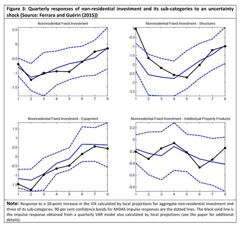
As for the effects on quarterly investment, we look at various non-residential investment sub-categories. We find that the most irreversible investment category (investment in structures) reacts the most negatively to uncertainty shocks as opposed to investment in intellectual property products that do not react much in the wake of uncertainty shocks (Figure 3). This matches well with intuition, since in a highly uncertain environment, the most costly projects with the most distant return prospects are likely to be the first investment plans to be sidelined given that they cannot be easily undone.



Overall, a number of policy implications can be drawn from our analysis. First, to the extent that uncertainty shocks are not protracted, there is no disproportionate impact attached to high-frequency (daily) uncertainty shocks in that they yield similar responses than same-size low-frequency shocks. Hence, on average, one should not worry too much about the consequences of a temporary (i.e., daily or weekly) spike in volatility for the macroeconomic environment. Second, given that we find that investment in structures reacts the most to uncertainty shocks, this suggests that policy interventions designed to boost investment in the wake of uncertainty shocks should concentrate in priority on infrastructure investment.

This post written by Laurent Ferrara and Pierre Guérin.

Anil Kashyap on the Greek crisis

University of Chicago Professor Anil Kashyap has a helpful summary of the Greek financial crisis.

Our distant neighbors

There’ve been some stunning pictures recently sent back from distant parts of our solar system which I wanted to share.

When I was a boy, people could only imagine what a comet actually looks like. Now we know.

Comet 67P/Churyumov-Gerasimenko as seen from 86 kilometers by European Space Agency Rosetta mission in March 2015. Image courtesy of ESA/Rosetta/NAVCAM.

NASA’s Dawn probe, launched from earth in 2007, this month sent back some phenomenal pictures of the dwarf planet Ceres, whose 1000 km diameter makes it the largest object in the asteroid belt. Remarkable features include some extremely bright reflective areas and a 3-mile-high pyramid.

Bright spots on dwarf planet Ceres. Image courtesy of NASA/JPL-Caltech/UCLA/MPS/DLR/IDA.

Pyramid structure on dwarf planet Ceres. Image courtesy of NASA/JPL-Caltech/UCLA/MPS/DLR/IDA.

Jupiter’s moon Europa, despite being stuck a frigid 3/4 of a billion kilometers away from the sun, is now believed to hold a liquid ocean of water beneath its icy crust, kept warm by the tidal forces of the gravitational pull from the giant planet. And perhaps life in those oceans? You can bet I’m a big supporter of NASA’s plans for a new mission to see what’s there.

Realistic color image of Europa constructed from mosaic of images taken by NASA’s Galileo Probe. Surface is mostly water ice with red-brown cracks and ridges containing significant amounts of other materials. Image courtesy of NASA/JPL-Caltech/SETI Institute.

Saturn’s moon Titan definitely has clouds that rain down on surface oceans. But its weather patterns are based on liquid methane, not H20.

Clouds moving over the Ligeia Mare, a large methane sea of Titan, based on images taken by the Cassini orbiter. Image courtesy of NASA/JPL-Caltech/Space Science Institute.

Geysers spewing water ice out from Enceladus, another of Saturn’s many moons, appear to be the source of one of the giant planet’s beautiful rings.

Geyser basin on Enceladus as seen from Cassini. Image courtesy of NASA/JPL-Caltech/Space Science Institute.

Like many others of my generation, I was sad to see Pluto demoted from its long-held status as our solar system’s ninth planet. But that disappointment is made up for by the remarkable recent images from NASA’s New Horizons probe of Pluto and its moon Charon in their orbital dance. Can’t wait to see the close-ups.

Week-long time-lapse pictures of Pluto and Charon taken from 100 million kilometers away by New Horizons. Image courtesy of NASA/Johns Hopkins University Applied Physics Laboratory/Southwest Research Institute.