Nate Silver's Blog, page 41

Politics Podcast: Michelle Obama Ripped President Trump On Night One Of The Convention

By Galen Druke, Clare Malone, Perry Bacon Jr. and Nate Silver, Galen Druke, Clare Malone, Perry Bacon Jr. and Nate Silver, Galen Druke, Clare Malone, Perry Bacon Jr. and Nate Silver and Galen Druke, Clare Malone, Perry Bacon Jr. and Nate Silver












 












More: Apple Podcasts |
ESPN App |
RSS

Late Monday, the FiveThirtyEight Politics podcast crew reacted to the first night of the virtual Democratic National Convention. Former First Lady Michelle Obama criticized President Trump forcefully, and a variety of politicians called for unity behind Joe Biden.

You can listen to the episode by clicking the “play” button in the audio player above or by downloading it in iTunes , the ESPN App or your favorite podcast platform. If you are new to podcasts, learn how to listen .

The FiveThirtyEight Politics podcast is recorded Mondays and Thursdays. Help new listeners discover the show by leaving us a rating and review on iTunes . Have a comment, question or suggestion for “good polling vs. bad polling”? Get in touch by email, on Twitter or in the comments.

Do You Buy That … Trump Still Has A Clear Path To Re-election?

Our Election Forecast Didn’t Say What I Thought It Would

My editors are forever asking me to take the long Twitter threads I write and turn them into articles here at FiveThirtyEight. So I’m actually going to give that a try!

What follows are some follow-up thoughts on our election model, which was originally composed in the form of a V E R Y L O N G tweetstorm that I never published. (See if you can guess where the 240-character breaks would have been.)

In this thread … err, article … I’ll try to walk you through my thought process on a few elements of our model and respond to a few thoughtful critiques I’ve seen elsewhere. Before you dive in, it may help to read our summary of the state of the race, or at least skim our very detailed methodology guide.

But the basic starting point for a probabilistic, poll-driven model ought to be this: Is polling in August a highly reliable way to predict the outcome in November?

The short answer is “no.”

Polling in August is somewhat predictive. You’d much rather be ahead than behind. But there can still be some very wild swings.

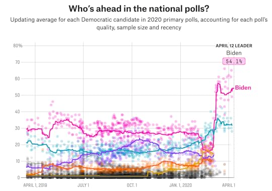
You can see that in the daily threads that Nathaniel Rakich, one of our elections analysts, puts together. Here is what a national polling average would have looked like in elections dating back to 1976:

The @FiveThirtyEight nat'l polling average with 84 days until E-Day:

2020: Biden+8.3
2016: Clinton+6.6
2012: Obama+0.5
2008: Obama+2.6
2004: Kerry+2.5
2000: Bush+10.0
1996: Clinton+11.3
1992: Clinton+20.1
1988: Dukakis+5.6
1984: Reagan+16.0
1980: Reagan+22.1
1976: Carter+26.6

— Nathaniel Rakich (@baseballot) August 11, 2020

OK, I cheated a bit. I’m using a version that Nathaniel published last week, partly because this was the exact moment in the campaign when Michael Dukakis, the 1988 Democratic nominee, started to blow his large lead, which he never regained. Still, there’s some wild stuff there! John Kerry led at this point in 2004. George W. Bush had a 10-point lead at this point in the 2000 race, but, as we know, he didn’t win the popular vote that year. In other cases, the leading candidate won, but the margin was off by as much as 20 points (Jimmy Carter in 1976).

Now, as I wrote last week, there are some caveats here. Several of these polling averages were taken while one or both candidates were experiencing convention bonuses, and although there are ways to correct for those, every time you correct for something so your model fits the past data better, you raise the possibility that you’re overfitting the data and that your model won’t be as accurate as claimed when applied to situations where you don’t already know the outcome.

There are also decent arguments that polling averages have become more stable in recent years. In that case, the wild fluctuations in the polls from, say, 1976 or 1988 might not be as relevant.

Our model actually agrees with these theories, up to a point! The fact that voters are more polarized now (more polarization means fewer swing voters, which means less volatility) is encoded into our model as part of our “uncertainty index,” for instance.

But we think it’s pretty dangerous to go all in on these theories and assume that poll volatility is necessarily much lower than it was before. For one thing, the theory is not based on a ton of data. Take the five most recent elections, for instance. The 20041 and 2012 elections featured highly stable polling — 2012 especially so. But 2000 and 2016 (!) did not, and 2008 election polling was not especially stable, either. Small sample sizes are already an issue in election forecasting, so it seems risky to come to too many firm conclusions about polling volatility based on what amounts to two or three examples.

Meanwhile, other people have pointed out that the most recent two presidents, Trump and Barack Obama, have had highly stable approval ratings. But the president just before them, George W. Bush, did not. His approval rating went through some of the wildest fluctuations ever, in fact, even though polarization was also fairly high from 2000 to 2008.

That said, polls have been stable so far this year. Indeed, that’s another factor that our uncertainty index accounts for. But don’t get too carried away extrapolating from this stability. Case in point: Polls were extremely stable throughout most of the Democratic primaries … but when the voting started, we saw huge swings from the Iowa caucuses through Super Tuesday. Poll volatility tends to predict future volatility, but only up to a point.

Remember, too, that voters haven’t yet been exposed to the traditional set pieces of the campaign, namely the conventions and the debates, which are often associated with higher volatility.

Now, suppose that despite all the weirdness to come in the general election campaign, Biden just plows through, leads by 6 to 9 points the whole way … and then wins by that amount on Nov. 3? If that happens, then we’ve got more evidence for the hypothesis that elections have become more stable, even when voters are confronted with a lot of surprising news.

But, crucially, we don’t have that evidence yet. So some of the models that are more confident in Biden’s chances seem to be begging the question, presuming that polls will remain stable when I’m not sure we can say that yet.

Then there’s the issue of COVID-19. Sometimes — though people may not say this outright — you’ll get a sense that critics think it’s sort of cheating for a model to account for COVID-19 because it’s never happened before, so it’s too ad hoc to adjust for it now.

I don’t really agree. Models should reflect the real world, and COVID-19 is a big part of the real world in 2020. Given the choice between mild ad-hockery and ignoring COVID-19 entirely, I think mild ad-hockery is better.

However, I also think there are good ways to account for COVID-19 without being particularly ad hoc about it. If you’re designing a model, whenever you encounter an outlier or an edge case or a new complication, the question you ask yourself should be, “What lessons can I draw from this that generalize well?” That is: Are there things you can do to handle the edge case well that will also make your model more robust overall?

As an aside, when testing models on historical data I think people should pay a lot of attention to edge cases and outliers. For instance, I pay a lot of attention to how our model is handling Washington, D.C. Why Washington? Well, if you take certain shortcuts — don’t account for the fact that vote shares are constrained between 0 and 100 percent of the vote — you might wind up with impossible results, like Biden winning 105 percent of the vote there. Or when designing an NBA model, I may pay a lot of attention to a player like Russell Westbrook, who has long caused issues for statistical systems. I don’t like taking shortcuts in models; I think they come back to bite you later in ways you don’t necessarily anticipate. But if you can handle the outliers well, you’ve probably built a mathematically elegant model that works well under ordinary circumstances, too.

But back to COVID-19: What this pandemic encouraged us to do was to think even more deeply about the sources of uncertainty in our forecast. That led to the development of the aforementioned uncertainty index, which has eight components (described in more depth in our methodology post):

The number of undecided voters in national polls. More undecided voters means more uncertainty.
The number of undecided plus third-party voters in national polls. More third-party voters means more uncertainty.
Polarization, as measured elsewhere in the model, which is based on how far apart the parties are in roll call votes cast in the U.S. House. More polarization means less uncertainty since there are fewer swing voters.
The volatility of the national polling average. Volatility tends to predict itself, so a stable polling average tends to remain stable.
The overall volume of national polling. More polling means less uncertainty.
The magnitude of the difference between the polling-based national snapshot and the fundamentals forecast. A wider gap means more uncertainty.
The standard deviation of the component variables used in the FiveThirtyEight economic index. More economic volatility means more overall uncertainty in the forecast.
The volume of major news, as measured by the number of full-width New York Times headlines in the past 500 days, with more recent days weighted more heavily. More news means more uncertainty.

Previous versions of our model had basically just accounted for factors 1 and 2 (undecided and third-party voters), so there are quite a few new factors here. And indeed, factors 7 and 8 are very high thanks to COVID-19 and, therefore, boost our uncertainty measure. However, we’re also considering several factors for the first time (like polarization and poll volatility) that reduce uncertainty.

In the end, though, our model isn’t even saying that the uncertainty is especially high this year. The uncertainty index would have been considerably higher in 1980, for instance. Rather, this year’s uncertainty is about average, which means that the historical accuracy of polls in past campaigns is a reasonably good guide to how accurate they are this year. That seems to me like a pretty good gut check.

It might seem counterintuitive that uncertainty would be about average in such a weird year, but accounting for multiple types of uncertainty means that some can work to balance each other out. We don’t have a large sample of elections to begin with; depending on how you count, somewhere between 10 and 15 past presidential races had reasonably frequent polling. So your default position might be that you should use all of that data to calibrate your estimates of uncertainty, rather than to try to predict under which conditions polls might be more or less reliable. If you are going to try to fine-tune your margin of error, though, then we think you need to be pretty exhaustive about thinking through sources of uncertainty. Accounting for greater polarization but not the additional disruptions brought about by the pandemic would be a mistake, we think; likewise, so would be considering the pandemic but not accounting for polarization.

I’ve also seen some objections to the particular variables we’ve included in the uncertainty index. For instance, not everybody likes that our way of specifying “the volume of major news” is based on New York Times headlines. I agree that this isn’t ideal. The New York Times takes its headlining choices very seriously, but as we learned from thumbing through years of its headlines, it also makes some idiosyncratic choices.

However, I don’t think anybody would say there hasn’t been a ton of important news this year, much of which could continue to reverberate later in the race. Nor should people doubt that poll volatility is often news-driven. Polls generally don’t move on their own, but rather in response to major political events (such as debates) and news events (such as wars starting or ending). Even before COVID-19, we were trying to incorporate some of this logic into our polling averages by, for instance, having them move more aggressively after debates.

Other people have suggested that we ought to have accounted for incumbency in the uncertainty index, on the theory that when incumbents are running for reelection, they are known commodities, which should reduce volatility. That’s a smart suggestion, and something I wish I’d thought to look at, although after taking a very brief glance at it now, I’m not sure how much it would have mattered. The 1980 and 1992 elections, which featured incumbents, were notably volatile, for instance.

So if it’s too soon to be all that confident that Biden will win based on the polls — not that a 71 percent of winning the Electoral College (and an 82 percent chance of winning the popular vote) are anything to sneeze at — is there anything else that might justify that confidence?

In our view, not really.

I’ll be briefer on these points, since we covered them at length in our introductory feature. But forecasts based on economic “fundamentals” — which have never been as accurate as claimed — are a mess this year. Depending on which variables you look at (gross domestic product or disposable income?) and over what time period (third quarter or second quarter?) you could predict anything from the most epic Biden landslide in the history of elections to a big Trump win.

Furthermore, FiveThirtyEight’s version of a fundamentals model actually shows the race as a tie — it expects the race to tighten given the high polarization and projected economic improvement between now and November. So although we don’t weigh the fundamentals all that much, they aren’t exactly a reason to be more confident in Biden.

What about Trump’s approval rating? It’s been poor for a long time, obviously. And some other models do use it as part of their fundamentals calculation. But I have trouble with that for two reasons. First, the idea behind the fundamentals is that they’re … well, fundamental, meaning they’re the underlying factors (like economic conditions and political polarization) that drive political outcomes. An approval rating, on the other hand, should really be the result of those conditions.

Second, especially against a well-known opponent like Biden, approval ratings are largely redundant with the polls. That is to say, if Trump’s net approval rating (favorable rating minus unfavorable rating) is -12 or -13 in polls of registered and likely voters, then his being down 8 or 9 points in head-to-head polls against Biden is pretty much exactly what you’d expect. (Empirically, though, the spread in approval ratings are a bit wider than the spreads in head-to-head polls. A candidate with a -20 approval rating, like Carter had at the end of the 1980 campaign, wouldn’t expect to lose the election by 20 points.)

Also, models that include a lot of highly correlated variables can have serious problems, and approval ratings and head-to-head polls are very highly correlated. I’m not saying you couldn’t work your way around these issues, but unless you were very careful, they could lead to underestimates of out-of-sample errors and other problems.

One last topic: the role of intuition when building an election model. To the largest extent possible, when I build election models, I try to do it “blindfolded,” by which I mean I make as many decisions as possible about the structure of the model before seeing what the model would say about the current year’s election. That’s not to say we don’t kick the tires on a few things at the end, but it’s pretty minimal, and it’s mostly to look at bugs and edge cases rather than to change our underlying assumptions. The process is designed to limit the role my priors play when building a model.

Sometimes, though, when we do our first real model run, the results come close to my intuition anyway. But this year they didn’t. I was pretty sure we’d have Biden with at least a 75 percent chance of winning and perhaps as high as a 90 percent chance. Instead, our initial tests had Biden with about a 70 percent chance, and he stayed there until we launched the model.

Why was my intuition wrong? I suspect because it was conditioned on recent elections where polls were fairly stable — and where the races were also mostly close, making Biden’s 8-point lead look humongous by comparison. If I had vividly remembered Dukakis blowing his big lead in 1988, when I was 10 years old, maybe my priors would have been different.

But as I said earlier, I’m not necessarily sure we can expect the polls to be quite so stable this time around. And when you actually check how accurate summer polling has been historically, it yields some pretty wide margins of error.

Nate Silver Introduces The 2020 Election Forecast

Animation by Luis Yordan

FiveThirtyEight editor-in-chief Nate Silver walks us through the 2020 Presidential Election Forecast. Learn how to navigate the new model — and find out what to keep an eye on as Election Day approaches.

Model Talk: How The 2020 Presidential Forecast Works

FiveThirtyEight’s 2020 presidential election forecast is live! In this edition of “Model Talk,” Nate Silver and Galen Druke break down what’s new in this year’s forecast and discuss where the uncertainty lies.

Politics Podcast: The 2020 Presidential Forecast Is Live!

By Galen Druke and Nate Silver and Galen Druke and Nate Silver












 












More: Apple Podcasts |
ESPN App |
RSS

On Wednesday, we launched our 2020 presidential election forecast. It currently shows Joe Biden with a 71 percent chance of winning the election and President Trump with a 29 percent chance. In this “Model Talk” edition of the FiveThirtyEight Politics podcast, Nate Silver and Galen Druke discuss the new additions to the forecast and what makes this election’s outcome so uncertain.

You can listen to the episode by clicking the “play” button in the audio player above or by downloading it in iTunes , the ESPN App or your favorite podcast platform. If you are new to podcasts, learn how to listen .

The FiveThirtyEight Politics podcast is recorded Mondays and Thursdays. Help new listeners discover the show by leaving us a rating and review on iTunes . Have a comment, question or suggestion for “good polling vs. bad polling”? Get in touch by email, on Twitter or in the comments.

2020 Election Forecast

National overviewNational overviewArizonaColoradoFloridaGeorgiaIowaMaine (statewide)MichiganMinnesotaNevadaNew HampshireNew MexicoNorth CarolinaOhioPennsylvaniaVirginiaWisconsinAlabamaAlaskaArizonaArkansasCaliforniaColoradoConnecticutDelawareDistrict of ColumbiaFloridaGeorgiaHawaiiIdahoIllinoisIndianaIowaKansasKentuckyLouisianaMaine (statewide)Maine 1st DistrictMaine 2nd DistrictMarylandMassachusettsMichiganMinnesotaMississippiMissouriMontanaNebraska (statewide)Nebraska 1st DistrictNebraska 2nd DistrictNebraska 3rd DistrictNevadaNew HampshireNew JerseyNew MexicoNew YorkNorth CarolinaNorth DakotaOhioOklahomaOregonPennsylvaniaRhode IslandSouth CarolinaSouth DakotaTennesseeTexasUtahVermontVirginiaWashingtonWest VirginiaWisconsinWyoming hey there! I’m Fivey Fox, and I’m here to show you around. Each of these maps is an example of how things might shake out on Election Day.

Latest news

MAY 4, 2020

The race for the presidency is not officially over, but in lots of ways the contest has been resolved. Maine’s 2nd district is heating up and we’re also keeping an eye on Utah’s 1st.

The former vice president Joseph R. Biden Jr. has amassed hundreds more delegates than the senator from Vermont, building an advantage that is all but insurmountable.
The only other candidate who was still running, Tulsi Gabbard, dropped out and endorsed Mr. Biden.

2020 ELECTION COVERAGE

Will Justin Amash’s Presidential Run Help Or Hurt Trump?

By Geoffrey Skelley and Tony Chow

What Went Down In Ohio’s Primary

By Nathaniel Rakich

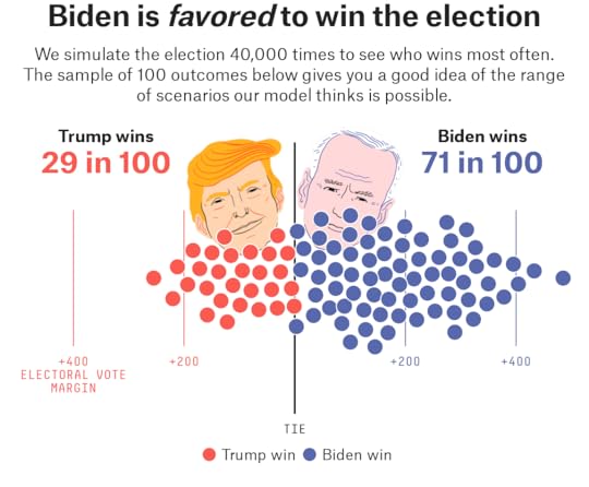
To put all these numbers in context, check out our coverage and subscribe to the FiveThirtyEight Politics podcast!Biden is favored to win the election

We simulate the election 40,000 times to see who wins most often. The sample of 100 outcomes below gives you a good idea of the range of scenarios our model thinks is possible.

TIE 400ELECTORALVOTES 200 200 40028 in 10028 in 100Trump winsTrump wins72 in 10072 in 100Biden winsBiden winsTrump winBiden win

Don’t count the underdog out! Upset wins are surprising but not impossible.Every outcome in our simulations

All possible Electoral College outcomes for each candidate, with higher bars showing outcomes that appeared more often in our 40,000 simulations

0100200300400500270 ELECTORAL VOTESSmoothedrollingaverageTrumpTrumpwinswinsMorelikelyMorelikely0100200300400500BidenBidenwinswinsMore bars to the right of the 270 line means more simulations where that candidate wins. Some of the bars represent really weird outcomes, but you never know!The winding path to victory

States that are forecasted to vote for one candidate by a big margin are at the ends of the path, while tighter races are in the middle. Bigger segments mean more Electoral College votes. Trace the path from either end to see which state could put one candidate over the top.

VOTE MARGINSTIPPING POINTS270 ELECTORAL VOTESNE3WYWVIDOKLAHOMANDSDALABAMAKENTUCKYNEUTAHTENNESSEELOUISIANAARKANSASNE1INDIANAKANSASMTMISSISSIPPIMISSOURIAKSOUTH CAROLINATEXASIOWAME2GEORGIAOHIONORTH CAROLINAARIZONANE2FLORIDAWISCONSINPENNSYLVANIAMINNESOTANEVADANHMICHIGANMECOLORADOVIRGINIANMOREGONNEW JERSEYCONNECTICUTME1ILLINOISDERIWASHINGTONNEW YORKMARYLANDCALIFORNIAMASSACHUSETTSHIVTDCMaine and Nebraska’s congressional districts are shown separately because those states split their Electoral College votes, allotting some to the statewide winner and some to the winner of each district.We call this the

How FiveThirtyEight’s 2020 Presidential Forecast Works — And What’s Different Because Of COVID-19

Our presidential forecast, which launched today, is not the first election forecast that FiveThirtyEight has published since 2016. There was our midterms forecast in 2018, which was pretty accurate in predicting the makeup of the House and the Senate. And there was our presidential primaries model earlier this year, which was a bit of an adventure but mostly notable for being bullish (correctly) on Joe Biden and (incorrectly) on Bernie Sanders. But we’re aware that the publication of our first presidential forecast since 2016 is liable to be fraught.

We’d like to address one thing upfront, though: We think our model did a good job in 2016. Although it had Hillary Clinton favored, it gave Donald Trump around a 30 percent chance of winning on Election Day,1 which was considerably higher than other models, prediction markets, or the conventional wisdom about the race. Moreover, the reasons the model was more bullish on Trump than other forecasts — such as detecting a potential overperformance for Trump in the Electoral College – proved to be important to the outcome.

Also, we’ve found that FiveThirtyEight’s models — including our election forecasts since they were first published in 2008 — have been well calibrated over time. Candidates whom our models claim have a 30 percent chance of winning really do win their races about 30 percent of the time, for example.

So if this were an ordinary election, we’d probably just say screw it, take the 2016 version of our model, make some modest improvements, and press “go.” We’d certainly devote more attention to how the model was presented, but the underlying math behind it would be about the same.

We are not so sure that this is an ordinary election, though. Rather, it is being contested amidst the most serious pandemic to hit the United States since 1918. So we’ve been doing a lot of thinking about how COVID-19 and other news developments could affect various aspects of the race, ranging from its impact on the economy to how it could alter the actual process of voting.

Put another way, while we think “ZOMG 2016!!!” is not a good reason to rethink a model that tended to be pretty cautious in the first place, we think COVID-19 might be.

What’s different from 2016

In the end, our model still isn’t that different from 2016’s, but let’s run through the list of changes. After that, we’ll provide a front-to-back description of how our model works.

First, a number of changes in the model are related to COVID-19:

In forecasting how much the polls could change, we now account for more components related to uncertainty. Two of these components include estimating i) economic uncertainty and ii) the overall volume of important news, both of which are very high under COVID-19. These offset other trends — such as greater polarization — that would lead to less uncertainty.
We’ve put a lot more work into our economic index: i) extending it back to 1880 to capture a fuller range of economic conditions, ii) adjusting it for increased partisanship and iii) developing an economic forecasting component to reflect potential changes in the economy between now and November. This is important because most projections forecast substantial improvement in the economy before November.
We attempt to account for additional uncertainty in Election Day results because turnout will potentially be less predictable given the pandemic.
We allow COVID-19 to be a factor in determining covariance. That is to say, states that have had high rates of COVID deaths and cases (such as Arizona and New York, which otherwise don’t have that much in common politically) could have correlated outcomes. Likewise, we also consider covariance based on a state’s anticipated rate of mail voting.
With the party conventions being substantially scaled down and largely held virtually, we’re applying only half of the usual “convention bounce adjustment” (see below for more on the convention bounce adjustment).

Other changes fall more into the category of continual improvements we’re making to our models that aren’t directly related to COVID-19:

Since 2016, we’ve made various changes to how our polling averages are calculated, as described here.
We now account for changes in how easy it is to vote in each state, as empirically, this yields higher turnout and a higher share of Democratic votes.
The model is now more careful around major events such as presidential debates that can have an outsize impact on candidates’ polling averages. If a candidate gains ground in the polls following one of these events, he will have to sustain that movement for a week or two to get full credit for it.
We’re running only one version of the presidential model this year. Things are complicated enough in an election held during a pandemic without getting into “polls-only” and “polls-plus” forecasts. Nor is there a “now-cast.” Our polling averages are the best way to reflect the current snapshot of the race, but the snapshot is not the same as the projected Election Day outcome.

The rest of how our model works involves three major steps. What follows is a pretty detailed walk-through, but I’ll be more circumspect when discussing steps described at more length elsewhere, such as in our 2016 methodology guide.

Step 1: Collect, analyze and adjust polls

Our national and state polling averages, which we began publishing in June, are the first steps we take in building our election forecast. We detailed our process for constructing those polling averages when we released them, so I’ll just review the highlights here.

Our polling averages are intended to be as inclusive as possible. We don’t want to have to make a lot of arbitrary decisions on which polls to include. But please review our polls policy for some exceptions on when we can’t use a poll in our forecast. Sometimes there are also delays in adding a poll until we can get more information about it.
Polls are weighted based on their sample size and their pollster rating, so higher-quality polls have more influence on the forecast. And if there are a large number of polls from one polling firm, the weight applied to each individual poll is discounted so no one pollster dominates the average.
Our polling averages reflect a blend of two methods. The first is a relatively simple weighted average, and the second is a more complicated method based on calculating a trend line. Of the two, the trend line method tends to be more aggressive. So early on in the campaign, we rely mostly on the more conservative weighted average method, while in the final few weeks, we mostly use the trend line method — that means our polling averages become more aggressive as Election Day nears.
The polling averages are subject to three types of adjustments:

The likely voter adjustment, which reflects that polls of likely voters and registered voters differ in predictable ways, adjusts polls of registered voters2 to make them more comparable to likely voter polls. Generally speaking, this means that Republicans (such as Trump) gain ground relative to Democrats when applying a likely voter screen, although this effect is mitigated when the Republican is an incumbent. Indeed, polls this year that have both a registered voter and likely voter version usually show Trump doing slightly better in the likely voter version. However, he does only modestly better, gaining around 1 percentage point on average.
The house effects adjustment, which detects polls that consistently lean toward one party or that consistently have more (or fewer) undecided voters than other polls of the same states, and adjusts them to correct for this. For example, Rasmussen Reports polls typically have very Republican-leaning results. So this adjustment would account for that. However, polls are allowed to retain at least some of their house effect, since an apparent house effect over a small number of polls could reflect statistical noise. In calculating house effects, the model mostly uses polls from the same state, so a polling firm could theoretically have a Trump-leaning house effect in one state and a Biden-leaning house effect in another.
Finally, we apply a timeline adjustment, which is based on a poll’s recency, and adjusts “old” polls for shifts in the overall race since it was conducted. For instance, say a poll of Arizona last month showed Biden up 3 points there, but there’s been a strong shift toward Trump since then in national polls and polls of similar states such as Nevada. This adjustment would shift that older Arizona poll toward Trump.

As we noted, the calculation of the polling averages is the first step in calculating our forecast. But they are not the same thing.

One time when this distinction is particularly relevant is following major events such as the debates and party conventions. These events sometimes produce big swings in the polls, and our polling averages are designed to be aggressive following these events and reflect the changed state of the race. However, these shifts are not necessarily long-lasting, and after a couple of weeks, the polls sometimes revert to where they were before.

Therefore, the model relies only partly on the polling average of the race after one of these events happens. For instance, say there is a debate on Oct. 1 and you’re looking at the model on, for example, Oct. 5. It will use a blend of the post-debate polling average from Oct. 5 and the pre-debate polling average from Oct. 1. After a week or two (depending on the event) though, the model will fully use the post-event polling average because it no longer necessarily expects a reversion to the mean.

In addition, our presidential model has traditionally applied a convention bounce adjustment that reflects the predictable boost in the polls that a party tends to get following its convention. Clinton surged to some of her biggest leads of the cycle following the Democratic Convention in 2016, for example. However, three factors could mitigate the convention bounce this year.

First, convention bounces have become smaller over time, likely reflecting a reduced number of swing voters because of greater partisanship. Based on current levels of polarization, for instance, we would expect a party to poll about 5 percentage points better at the peak of its convention bounce on the day just after the conclusion of its convention, with the effects fading fairly quickly thereafter. This is down from past convention bounces that could sometimes be measured in the double digits.
Second, as mentioned before, we are applying only half of the usual convention bounce adjustment this year because due to COVID-19, the conventions are being scaled back.
Third, because this year’s Republican National Convention occurs the week immediately following the Demoratic National Convention, the effects could largely cancel each other out — Biden’s bounce could be derailed by Trump’s bounce, in other words. Because Trump’s convention occurs second, the effects of it might linger for slightly longer, but the model expects the net effect to be small given that the Democratic convention will also be fairly fresh in voters’ minds.

Thus, the convention bounce adjustments will be small this year. Polls conducted in the period between the Democratic convention and the Republican convention will be adjusted toward Trump by around 2 or 2.5 percentage points, depending on the precise dates of the polls. And polls in the two to three weeks after the Republican convention will be adjusted toward Biden but only very slightly so (by less than 1 full percentage point).

Step 2: Combine polls with “fundamentals,” such as demographic and economic data

As compared with other models, FiveThirtyEight’s forecast relies heavily on polls. We do, however, incorporate other data in two main ways:

First, the polling average in each state is combined with a modeled estimate of the vote based on demographics and past voting patterns to create what we call an “enhanced snapshot” of current conditions. This is especially important in states where there is little or no polling.
Second, that snapshot is then combined with our priors, based on incumbency and economic conditions, to create a forecast of the Election Day outcome.

Enhancing our polling averages

At the core of the modeled estimate is FiveThirtyEight’s partisan lean index, which reflects how the state voted in the past two presidential elections as compared with the national average. In our partisan lean index, 75 percent of the weight is assigned to 2016 and 25 percent to 2012. So note, for example, that Ohio (which turned much redder between 2012 and 2016) is not necessarily expected to continue to become redder. Instead, it might revert somewhat to the mean and become more purple again.

The partisan lean index also contains a number of other adjustments:

We adjust for the home states of the presidential and vice presidential candidates. The size of the home-state adjustment is much larger for presidential candidates than for their running mates. The size of the state is also a factor: Home-state advantages are larger in states with smaller populations. We also allow candidates to be associated with more than one state, in which case the home-state bonus is divided. For Biden, for instance, his primary home state is Delaware (where he lives now), and his secondary state is Pennsylvania (where he was born). And for Trump, his primary home state is New York (where he was born), and his secondary state is Florida (where he officially claims residence).3
We also adjust for what we call a state’s elasticity. Some states such as New Hampshire “swing” more than others in response to national trends because they have a higher proportion of swing voters, which can cause wider fluctuations from cycle to cycle. The elasticity scores we’re using for 2020 are based on a blend of each state’s elasticity in 2008, 2012 and 2016.
And finally, we account for changes in how easy it is to vote in each state based on the Cost of Voting Index, as researchers have found that states with higher barriers to voting tend to produce better results for Republican candidates and states with lower barriers tend to lean more Democratic.4

We then apply the partisan lean index in three slightly different ways to create a modeled estimate of the vote in each state.

First is what we call the “rigid method” because it rigidly follows the partisan lean index. In this technique, we first impute where the race stands nationally based on a blend of state and national polls. (Most of the weight in this calculation actually goes to state polls, though. National polls play relatively little role in the FiveThirtyEight forecast, other than to calculate the trend line adjustment in Step 1.) Then we add a state’s partisan lean index to it. For instance, if we estimate that Biden is ahead by 5 points nationally, and that a state’s partisan lean index is D 10 — meaning it votes 10 points more Democratic than the country as a whole — the rigid method would project that Biden is currently ahead by 15 points there.5
Second is the demographic regression method. Basically, the goal of this technique is to infer what the polls would say in a state based on the polls of other states that have more polling. In this method, adopted from a similar process we applied in our primary model, we use a state’s partisan lean index plus some combination of other variables in a series of regression analyses to try to fit to the current polling in each state. The variables considered include race (specified in several different ways), income, education, urbanization, religiosity6 and an index indicating the severity of the COVID-19 situation in each state, based on the number of cases and deaths per capita as recorded by the COVID Tracking Project. (Technically speaking, the model runs as many as 180 different regressions based on various combinations of these variables, but there are limits on which variables may appear in the regressions together in order to avoid collinearity, as well as how many variables can be included.) We then take a weighted average of all the regressions, where regression specifications with a higher adjusted R2 receive more weight but all regressions receive at least some weight.
Third is the regional regression method. This is much simpler: It consists of a single regression analysis where the dependent variables are a state’s partisan lean index, plus dummy variables indicating which of the four major regions (Northeast, Midwest, South, West) the state is in.7

We then combine these three estimates to create an ensemble forecast for each state. The rigid method, which is the most accurate historically, receives the majority of the weight, followed by the demographic regression and then the regional regression.

Then, we combine the ensemble forecast with a state’s polling average to create an enhanced snapshot of the current conditions in each state. The weight given to the polling average depends on the volume of polling in each state and how recently the last poll of the state was conducted. As of the forecast launch (Aug. 12), around 55 percent of the weight goes to the polling average rather than to the ensemble in the average state. However, in well-polled states toward the end of the campaign, as much as 97 or 98 percent of the weight could go toward the polling average. Conversely, states that have few polls rely mostly on the ensemble technique (and states that have no polls use the ensemble in lieu of a polling average).

Next, we combine the enhanced snapshots in each state to create a national snapshot, which is essentially our prediction of the national popular vote margin in an election held today. The national snapshot accounts for projected voter turnout in each state based on population growth since 2016, changes in how easy it is to vote since 2016, and how close the race is in that state currently — closer-polling states tend to have higher turnout. National polls are not used in the national snapshot; it’s simply a summation of the snapshots in the 50 states and Washington, D.C.

We know this is starting to get pretty involved — we’re really in the guts of the model now — but there is another important step. Our national snapshot is not the same thing as our prediction of the Election Day outcome. Instead, our prediction blends the polling-driven snapshot with a “fundamentals forecast” based on economic conditions and whether an incumbent is seeking reelection.

Polls vs. Fundamentals

I’m on the record as saying that I think presidential forecasting models based strictly on “fundamental” factors like economic conditions are overrated. Without getting too deep into the weeds, it’s easy to “p-hack” your way to glory with these models because there are so many ways to measure “the economy” but only a small sample size of elections for which we have reliable economic data. The telltale sign of these problems is that models claiming to predict past elections extremely well often produce inaccurate — or even ridiculous — answers when applied to elections in which the result is unknown ahead of time. One popular model based on second-quarter GDP, for example, implies that Biden is currently on track to win nearly 1,000 electoral votes — a bit of a problem since the maximum number theoretically achievable is 538.8

At the same time, that doesn’t mean the fundamentals are of no use at all. They can provide value and gently nudge your forecast in the right direction — if you use them carefully (although they’re hard to use carefully amidst something like the pandemic).

So, since 2012, we have used an index of economic conditions in our presidential forecast. In its current incarnation, it includes six variables:

Jobs, as indicated by nonfarm payrolls.
Spending, as indicated by real personal consumption expenditures.
Income, as measured by real disposable personal income.
Manufacturing, as measured by industrial production.
Inflation, based on the consumer price index.9
And the stock market, based on the S&P 500.

All variables are standardized so that they have roughly the same mean and standard deviation — and, therefore, have roughly equal influence on the index — for economic data since 1946. The index is then based on readings of these variables in the two years leading up to the election (e.g., from November 2018 through November 2020 for this election) but with a considerably heavier weight placed on the more recent data, in particular, the data roughly six months preceding the election. Where possible, the index is calibrated based on “vintage” economic data — that is, data as it was published in real time — rather than on data as later revised.

Although the quality of economic data is more questionable prior to the 1948 election, we have also attempted to create an approximate version of the index for elections going back to 1880 based on the data that we could find. (It’s extremely important, in our view, to expand the sample size for this sort of analysis, even if we have to rely on slightly less reliable data to do so.) Our economic index for elections dating to 1880 (see below) is expressed as a Z-score, where a score of zero reflects an average economy. And, as you can see, extremely negative economic conditions tend to predict doom for the incumbent party (as in 1932, 1980 and 2008).

The economy is a noisy predictor of presidential success

FiveThirtyEight’s economic index as of Election Day, since 1880,* where a score of zero reflects an average economy, a positive score a strong economy and a negative score a weak one

Year
Economic Index

Year
Economic Index




1880
1.37

1948
-0.29


1884
-0.18

1952
0.21


1888
-0.25

1956
0.07


1892
0.71

1960
-0.01


1896
-0.15

1964
0.70


1900
0.56

1968
0.23


1904
-0.23

1972
0.46


1908
-1.03

1976
0.26


1912
0.13

1980
-1.71


1916
0.75

1984
0.86


1920
-1.52

1988
0.09


1924
0.44

1992
-0.29


1928
0.15

1996
0.36


1932
-2.34

2000
0.36


1936
1.55

2004
0.01


1940
0.77

2008
-1.34


1944
1.01

2012
-0.10





2016
0.08

*Values prior to the 1948 election are based on more limited data and should be considered rough estimates.

But, overall, the relationship between economic conditions and the incumbent party’s performance is fairly noisy. In fact, we found that the economy explains only around 30 percent of the variation in the incumbent party’s performance, meaning that other factors explain the other 70 percent.

We do try to account for some of those “other” factors, although we’ve found they make only a modest difference. For instance, we also account for whether the president is an elected incumbent (like Trump this year or Barack Obama in 2012), an incumbent who followed the line of succession into office (like Gerald Ford in 1976) or if there is no incumbent at all (as in 2008 or 2016). We also account for polarization based on how far apart the parties are in roll call votes cast in the U.S. House. Periods of greater polarization (such as today in the U.S.) are associated with closer electoral margins and also smaller impacts of economic conditions and incumbency.

One additional complication is that the condition of the economy at any given moment prior to the election may not resemble what it eventually looks like in November, which is what our model tries to predict. Thus, the model makes a simple forecast for each of the six economic variables, which accounts for some mean-reversion, but is also based on the recent performance of the stock market (yes, it has some predictive power) and surveys of professional economists.10

Although we’ll discuss this at more length in the feature that accompanies our forecast launch, the fundamentals forecast is not necessarily as bad as you might think for Trump, despite awful numbers in categories such as GDP. One of the economic components that the model considers (income) has been strong thanks to government subsidies in the form of the CARES Act, for instance, and two others (inflation and the stock market) have been reasonably favorable, too.

In addition, Trump is an elected incumbent, the economy is expected to improve between the forecast launch (August 12) and November, and the polarized nature of the electorate limits the damage to him to some degree. Thus, one shouldn’t conclude that Trump is a huge underdog on the basis of the economy alone, although he’s also not a favorite to win reelection as elected incumbents typically are.

The closer to Election Day, the more our model relies on polls

Share of the weight assigned to polls and the “fundamentals,” by number of days until the election

Days until election
Polls
Fundamentals




0
100%
0%


5
97
3


10
94
6


25
89
11


50
84
16


75
79
21


100
74
26


150
65
35


200
57
43


250
47
53

However, our model assigns relatively little weight to the fundamentals forecast, and the weight will eventually decline to zero by Election Day. (Although the fundamentals forecast does do a good job of forecasting most recent elections, there are a lot more misses once you extend the analysis before 1948. So keep that in mind in the table, as the assigned weight is based on the entire data set.) Nonetheless, here is how much the model weights the fundamentals up until the election.

As of forecast launch in mid-August, for instance, the model assigns 77 percent of the weight to the polling-based snapshot and 23 percent of the weight to the fundamentals. In fact, the fundamentals actually help Trump at the margin (they aren’t good for him, but they’re better than his polls), so the model shifts the snapshot in each state slightly toward Trump in the forecast of the Election Day outcome. States with higher elasticity scores are shifted slightly more in this process.

Step 3: Account for uncertainty and simulate the election thousands of times

As complicated though it may seem, everything I’ve described up until this point is, in some sense, the easy part of developing our model. There’s no doubt that Biden is comfortably ahead as of the forecast launch in mid-August, for example, and the choices one makes in using different methods to average polls or combine them with other data isn’t likely to change that conclusion.

What’s trickier is figuring out how that translates into a probability of Biden or Trump winning the election. That’s what this section is about.

Before we proceed further, one disclaimer about the scope of the model: It seeks to reflect the vote as cast on Election Day, assuming that there are reasonable efforts to allow eligible citizens to vote and to count all legal ballots, and that electors are awarded to the popular-vote winner in each state. It does not account for the possibility of extraconstitutional shenanigans by Trump or by anyone else, such as trying to prevent mail ballots from being counted.

That does not mean it’s safe to assume these rules and norms will be respected. (If we were sure they would be respected, there wouldn’t be any need for this disclaimer!) But it’s just not in the purview of the sort of statistical analysis we conduct in our model to determine the likelihood they will or won’t be respected.

We do think, however, that well-constructed polls and models can provide a useful benchmark if any attempts to manipulate the election do occur. For instance, a candidate (in a state with incomplete results because mail ballots have yet to be counted) declaring themselves the winner in a state where the model had given them an 0.4 percent chance of winning would need to be regarded with more suspicion than one where they’d had a 40 percent chance going in (although a 40 percent chance of winning is by no means a sure thing either, obviously).

With that disclaimer out of the way, here are the four types of uncertainty that the model tries to account for:

National drift, or how much the overall national forecast could change between now and Election Day.
National Election Day error, or how much our final forecast of the national popular vote could be off on Election Day itself.
Correlated state error, which reflects errors that could occur across multiple states along geographic or regional lines — for instance, as was relevant in 2016, a systematic underperformance relative to polls for the Democratic candidate in the Midwest.
State-specific error, an error relative to our forecast that affects only one state.

The first type of error, national drift, is probably the most important one as of the launch — that is, the biggest reason Biden might not win despite currently enjoying a fairly wide lead in the polls is that the race could change between now and November.

National drift is calculated as follows:

Constant x (Days Until Election)^⅓ x Uncertainty Index

That is, it is a function of the cube root of the number of days until the election11 times the FiveThirtyEight Uncertainty Index, which I’ll describe in a moment. (Note that the use of the cube root implies that polls do not become more accurate at a linear rate, but rather that there is a sharp increase in accuracy toward the end of an election. Put another way, August is still early as far as polling goes.)

The uncertainty index is a new feature this year, although it reflects a number of things we did previously, such as accounting for the number of undecided voters. In the spirit of our economic index, it also contains a number of measures that are historically correlated with greater (or lesser) uncertainty but are also correlated with one another in complicated ways. And under circumstances like these (not to mention the small sample size of presidential elections), we think it is better to use an equally-weighted blend of all reasonable metrics rather than picking and choosing just one or two metrics.

The components of our uncertainty index are as follows:

The number of undecided voters in national polls. More undecided voters means more uncertainty.
The number of undecided plus third-party voters in national polls. More third-party voters means more uncertainty.
Polarization, as measured elsewhere in the model, is based on how far apart the parties are in roll call votes cast in the U.S. House. More polarization means less uncertainty since there are fewer swing voters.
The volatility of the national polling average. Volatility tends to predict itself, so a stable polling average tends to remain stable.
The overall volume of national polling. More polling means less uncertainty.
The magnitude of the difference between the polling-based national snapshot and the fundamentals forecast. A wider gap means more uncertainty.
The standard deviation of the component variables used in the FiveThirtyEight economic index. More economic volatility means more overall uncertainty in the forecast.
The volume of major news, as measured by the number of full-width New York Times headlines in the past 500 days, with more recent days weighted more heavily. More news means more uncertainty.

In 2020, measures No. 1 through 5 all imply below-average uncertainty. There aren’t many undecided voters, there are no major third-party candidates, polarization has been high and polls have been stable. Measure No. 6 suggests average uncertainty. But metrics No. 7 and 8 imply extremely high uncertainty; there has been a ton of news related to COVID-19 and other major stories, like the protests advocating for police reform in response to the death of George Floyd — not to mention the impeachment trial of Trump earlier this year. Likewise, there has been as much volatility in economic data as at any time since the Great Depression.

On the one hand, the sheer number of uncertainties unique to 2020 indicate the possibility of a volatile election, but on the other hand, there are also a number of measures that signal lower uncertainty, like a very stable polling average. So when we calculate the overall degree of uncertainty for 2020, our model’s best guess is that it is about average relative to elections since 1972. That average, of course, includes a number of volatile elections such as 1980, 1988 and 1992, where there were huge swings in the polls over the final few months of the campaign, along with elections such as 2004 and 2012 where polls were pretty stable. As voters consume even more economic- and pandemic-related news — and then experience events like the conventions and the debates — it’s not yet clear whether the polls will remain stable or begin to swing around more.

It’s also not entirely clear how this might all translate into the national Election Day error — that is, how far off the mark our final polling averages are — either. In calculating Election Day error, we use a different version of the uncertainty index that de-emphasizes components No. 6, 7 and 8, since those components pertain mostly to how much we expect the polls to change between now and the election, rather than the possibility of an Election Day misfire.

Still, our approach to calculating Election Day error is fairly conservative. In order to have a larger sample size, the calculation is based on the error in final polls in elections since 1936, rather than solely on more recent elections. While polls weren’t as far off the mark in 2016 as is generally reputed (national polls were fairly accurate, in fact), it’s also not clear that the extremely precise polls in the final weeks of 2004, 2008 and 2012 will be easy to replicate given the challenges in polling today. Given the small sample sizes, we also use a fat-tailed distribution for many of the error components, including the national Election Day error, to reflect the small — but not zero — possibility of a larger error than what we’ve seen historically.

There could also be some challenges related to polling during COVID-19. In primary elections conducted during the pandemic, for instance, turnout was hard to predict. In some ways, the pandemic makes voting easier (expanded options to vote by mail in many states), but it also makes it harder in other ways (it’s difficult to socially distance if you must vote in person).

This is a rough estimate because there are a lot of confounding variables — including the end of the competitive portion of the Democratic presidential primary — but we estimate that the variability in turnout was about 50 percent higher in primary elections conducted after the pandemic began in the U.S. than those conducted beforehand. Empirically, we know that states that experience a sharp change in turnout from one cycle to the next are harder to forecast, too. So we estimate that a 50 percent increase in error when predicting turnout will result in a 20 percent increase in error when predicting the share of the vote each party receives.

Therefore, we increase national Election Day error, correlated state error and state-specific error by 20 percent relative to their usual values because of how the coronavirus could affect turnout and the process of voting. Note that this still won’t be enough to cover extraordinary developments such as mail ballots being impounded. But it should help to reflect some of the additional challenges in polling and holding an election amidst a pandemic.

When it comes to simulating the election — we’re running 40,000 simulations each time the model is updated — the model first picks two random numbers to reflect national drift (how much the national forecast could change) and national Election Day error (how off our final forecast of the national popular vote could be) that are applied more or less uniformly12 to all states. However, even if you somehow magically knew what the final national popular vote would be, there would still be additional error at the state level. A uniform national swing would not have been enough to cost Clinton the Electoral College in 2016, for example. But underperformance relative to the polls concentrated in the Midwestern swing states did.

In fact, we estimate that at the end of the campaign, most of the error associated with state polling is likely to be correlated with errors in other states. That is to say, it is improbable that there would be a major polling error in Michigan that wouldn’t also be reflected in similar states such as Wisconsin and Ohio.

Therefore, to calculate correlated polling error, the model creates random permutations based on different demographic and geographic characteristics. In one simulation, for instance, Trump would do surprisingly well with Hispanic voters and thus overperform in states with large numbers of Hispanics. In another simulation, Biden would overperform his polls in states with large numbers of Catholics. The variables used in the simulations are as follows:

Race (white, Black, Hispanic, Asian)
Religion (evangelical Christians, mainline protestants, Catholic, Mormon, other religions, atheist/nonreligious)
A state’s partisan lean index in 2016 and in 2012
Latitude and longitude
Region (North, South, Midwest, West)
Urbanization
Median household income
Median age
Gender
Education (the share of the population with a bachelor’s degree or higher)
Immigration (the share of a state that is part of its voting-eligible population)
The COVID-19 severity index (see Step 2)
The share of a state’s vote that is expected to be cast by mail

One mathematical property of correlated polling errors is that states with demographics that resemble those of the country as a whole tend to have less polling error than those that don’t. Underestimating Biden’s standing among Mormons wouldn’t cause too many problems in a national poll, or in a poll of Florida, for example. But it could lead to a huge polling error in Utah. Put another way, states that are outliers based on some combination of the variables listed above tend to be harder to predict.

Finally, the model randomly applies some residual, state-specific error in each state. This tends to be relatively small, and is primarily a function of the volume of polling in each state, especially in states that have had no polling at all. If you’re wondering why Trump’s chances are higher than you might expect in Oregon, for example, it’s partly because there have been no polls there as of forecast launch.

Odds and ends

Whew — that’s pretty much it! But a few random bullet points that don’t fit neatly into the categories above.

The model accounts for the fact that Maine and Nebraska award one electoral vote each to the winner of each congressional district. In fact, these congressional districts have their own forecast pages, just as the states do. For the most part, though, the statewide forecasts in Maine and Nebraska just reflect the sum of the district forecasts. However, because not all polls provide district-level breakdowns in these states, the model also makes inferences from statewide polls of Maine and Nebraska, too. In total, the model calculates a forecast in 54 jurisdictions: the two congressional districts in Maine, the three in Nebraska, the other 48 states and Washington, D.C.
In 2016, as well as in backtesting the model in certain past years (i.e., 1980, 1992) we designated “major” third-party candidates such as Gary Johnson and Ross Perot. We defined major as (i) a candidate who is on the ballot almost everywhere, (ii) who is included in most polls and (iii) who usually polls in at least the mid-to-high single digits. There is no such candidate in 2020.
However, we do predict votes for “other” candidates in each state. The predictions are based on how many third-party candidates appear on the ballot in the state,13 whether write-in votes are permitted, how much of the vote a state has historically given to third-party candidates, and how competitive the state is (third-party candidates historically receive fewer votes in swing states).
Electoral College ties (269-269) are listed as such in the model output. This is a change from past years, where we used various methods to break the ties. We do not account for the possibility of faithless electors or candidates other than Trump and Biden winning electoral votes.

Got any other questions or see anything that looks wrong? Please drop us a line.

It’s Way Too Soon To Count Trump Out

Joe Biden currently has a robust lead in polls. If the election were held today, he might even win in a landslide, carrying not only traditional swing states such as Florida and Pennsylvania but potentially adding new states such as Georgia and Texas to the Democratic coalition.

But the election is not being held today. While the polls have been stable so far this year, it’s still only August. The debates and the conventions have yet to occur. Biden only named his running mate yesterday. And the campaign is being conducted amidst a pandemic the likes of which the United States has not seen in more than 100 years, which is also causing an unprecedented and volatile economy.

Nor has it been that uncommon, historically, for polls to shift fairly radically from mid-August until Election Day. Furthermore, there are some reasons to think the election will tighten, and President Trump is likely to have an advantage in a close election because of the Electoral College.

That, in a nutshell, is why the FiveThirtyEight presidential election forecast, which we launched today, still has Trump with a 29 percent chance of winning the Electoral College, despite his current deficit in the polls. This is considerably higher than some other forecasts, which put Trump’s chances at around 10 percent. Biden’s chances are 71 percent in the FiveThirtyEight forecast, conversely.14

If these numbers give you a sense of deja vu, it may be because they’re very similar to our final forecast in 2016 … when Trump also had a 29 percent chance of winning! (And Hillary Clinton had a 71 percent chance.) So if you’re not taking a 29 percent chance as a serious possibility, I’m not sure there’s much we can say at this point, although there’s a Zoom poker game that I’d be happy to invite you to.

One last parallel to 2016 — when some models gave Clinton as high as a 99 percent chance of winning — is that FiveThirtyEight’s forecast tends to be more conservative than others. (For a more complete description of our model, including how it is handling some complications related to COVID-19, please see our methodology guide.)

With that said, one shouldn’t get too carried away with the comparisons to four years ago. In 2016, the reason Trump had a pretty decent chance in our final forecast was mostly just because the polls were fairly close (despite the media narrative to the contrary), close enough that even a modest-sized polling error in the right group of states could be enough to give Trump a victory in the Electoral College.

The uncertainty in our current 2020 forecast, conversely, stems mostly from the fact that there’s still a long way to go until the election. Take what happens if we lie to our model and tell it that the election is going to be held today. It spits out that Biden has a 93 percent chance of winning. In other words, a Trump victory would require a much bigger polling error than what we saw in 2016.

Let’s briefly expand on the points I made above.

Biden’s lead is pretty impressive

In this article — partly as a corrective against what I see as overconfident assessments elsewhere — I’m mostly focused on the reasons why Trump’s chances are higher than they might appear. But we should be clear: Trump’s current position in the polls is poor.

Biden is currently ahead in our polling averages in Florida, Wisconsin, Michigan, Pennsylvania, Arizona, Ohio and in the second congressional district in Nebraska — all places that Clinton lost in 2016. If he won those states (and held the other states Clinton won), that would be enough to give him 352 electoral votes. He’s also within roughly 1 percentage point of Trump in Texas, Georgia, Iowa and Maine’s second congressional district. If he won those, too, he’d be up to a whopping 412 electoral votes.

It’s important to remember that the uncertainty in our forecast runs in both directions. There’s the chance that Trump could come back — but there’s also the chance that things could get really out of hand for him. Our model thinks there’s a 19 percent chance that Biden will win Alaska, for example, and a 13 percent chance that he will win South Carolina. The model also gives Biden a 30 percent chance of a double-digit win in the popular vote, which would be the first time that happened since 1984.

But there are downside scenarios for Biden.

Polls often change substantially between now and November

Every day, my colleague Nathaniel Rakich tweets out a list of what our national polling average would have looked like at this stage in past campaigns. And it can be a pretty wild ride. Here is Tuesday’s version, for instance.

The @FiveThirtyEight nat'l polling average with 84 days until E-Day:

2020: Biden+8.3
2016: Clinton+6.6
2012: Obama+0.5
2008: Obama+2.6
2004: Kerry+2.5
2000: Bush+10.0
1996: Clinton+11.3
1992: Clinton+20.1
1988: Dukakis+5.6
1984: Reagan+16.0
1980: Reagan+22.1
1976: Carter+26.6

— Nathaniel Rakich (@baseballot) August 11, 2020

Three of the candidates leading in national polls at this point — Michael Dukakis in 1988, George W. Bush in 2000, and John Kerry in 2004 — did not actually win the popular vote. Bush blew a 10-point lead, in fact, which is larger than Biden’s current advantage. (Luckily for Bush, he won the Electoral College.) In other cases, the polls at this point “called” the winner correctly, but the margins were way off. Jimmy Carter eventually beat Gerald Ford by just 2.1 percentage points — not the 26.6-point lead he had at this point in the campaign. Bill Clinton won by 5.6 points — not 20.1 points. And Barack Obama won a considerably more commanding victory in 2008 than polls at this point projected.

Now, there are some mitigating factors here. Some of these polls were taken at the height of a candidate’s convention bounce, although there are ways to try to correct for those. And in general, polls have become less volatile over time, probably because increased polarization means there are fewer swing voters than there once were. The polls have been particularly stable so far this year, in fact.

But while there are some factors that reduce uncertainty, there are other factors that increase it.

COVID-19 is a big reason to avoid feeling overly confident about the outcome

The COVID-19 pandemic has led to more than 150,000 fatalities and has upended pretty much every American’s life, and Trump’s approval ratings for his handling of it have been awful.

But to the extent this is an election about COVID-19, there’s the possibility that the situation could improve between now and November. Cases have recently begun to come down after an early-summer spike, and recent economic data has shown improvement there, too. There’s also the possibility that a vaccine could be approved — or rushed out — by November, though it’s highly unlikely it could be widely distributed by then.

How to account for this? No, we aren’t building a COVID-19 projection model. (It’s really hard.) But we have built an “uncertainty index” that essentially governs the margin of error in our forecast. It contains eight components, two of which are very high because of COVID-19. Specifically, these are the high volatility in recent economic data, and the volume of major news events, as measured by the number of full-width New York Times headlines. There’s more news this year — not just about COVID-19, but the protests around police brutality, Trump’s impeachment earlier this year, etc. — than in any recent election campaign.

We also expect turnout to be harder to predict this year based on primary elections held during the pandemic that had highly variable turnout — which, in turn, could lead to more polling error. So even if the polls don’t change that much between now and November, that could create some additional uncertainty on Election Day. See the methodology guide for more on how we handle COVID-19.

But the other components of the uncertainty index are low, pointing toward a stable campaign. For instance, polarization is high, poll movement so far has been limited, and there aren’t that many undecided voters; the index accounts for all of those things.

In fact, the uncertainty index points toward the overall uncertainty going into November being about average relative to past presidential campaigns. So our model isn’t necessarily saying that things are going to get crazy, although they could. But it’s also saying you shouldn’t necessarily expect highly stable campaigns like 2012 to be the new normal in the time of COVID-19. (And keep in mind that 2016 was a pretty volatile campaign, too, even without COVID-19.) Empirically, the polls can move quite a bit from August to November, more than you might expect intuitively!

There are some sources of uncertainty that the model doesn’t account for, however. We assume that there are reasonable efforts to allow eligible citizens to vote and to count all legal ballots, and that electors are awarded to the popular-vote winner in each state. The model also does not account for the possibility of extraconstitutional shenanigans by Trump or by anyone else, such as trying to prevent mail ballots from being counted.

It’s hard to know what the “fundamentals” say

I’ve long been critical of models that use economic “fundamentals” to try to predict election results, mostly because — although they claim to be highly precise — they haven’t actually been very good at predicting the outcome of an election where they don’t already know the results.

And those models are especially likely to have problems this year because of highly variable economic data. One model based on second quarter GDP projects Trump to win -453 (negative 453!) electoral votes, for example. But if you built a model based on third-quarter GDP, which is expected to be highly positive, it might predict a Trump landslide.

This isn’t to say that we don’t employ a fundamentals forecast of our own. We do, but it’s much less confident than others, and it receives relatively little weight in the overall forecast. It also isn’t currently that bad for Trump. In fact, it essentially predicts the popular vote to be roughly tied. Why?

Although three of the economic factors we use in the model (jobs, spending, manufacturing) have been terrible, a fourth component (income) has been very strong because of government subsidies in the form of the CARES Act, though that could change if stimulus payments lapse. The fifth and sixth components, inflation and the stock market, have also been reasonably favorable.
Most of the variables that declined are now improving, and are expected to continue to improve. (Our model projects what the economy will look like by November rather than relying on current data.)
High polarization potentially blunts the impact of a poor economy.
Trump is an elected incumbent, and elected incumbents are usually favored for reelection.
We extended our analysis back to elections since 1880 (!) to expand the sample size, and found the relationship between the economy and the election likely isn’t as strong as other models claim, anyway.

In other words, our forecast thinks it’s far from obvious that the economy will doom Trump, especially if he can tell a story of recovery by November. Indeed, Trump’s approval ratings on the economy are still fairly good, so our model seems to be doing a reasonably good job of capturing how voters actually feel about the economy.

Another way to look at it is that our model is just saying that, in a highly polarized environment, the race is more likely than not to tighten in the stretch run. Empirically, large leads like the one Biden has now tend to dissipate to some degree by Election Day. And if the race does tighten…

Trump appears to have an Electoral College advantage again

Our model says there’s an 81 percent chance that Biden wins the popular vote — compared to his 71 percent chance in the Electoral College. That means there’s about a 10 percent chance that Trump again wins the Electoral College despite losing the popular vote. (Conversely, the model puts the chance that Biden wins the Electoral College but loses the popular vote at only around 1 in 750.)

That reflects the fact that the tipping-point state — the state that would provide the decisive 270th electoral vote — is somewhat to the right of the national popular vote. More specifically, our projection as of Tuesday had Biden winning the popular vote by 6.3 percentage points nationally, but winning the tipping-point state, Wisconsin, by a smaller margin, 4.5 percentage points:

The Electoral College could once again help Trump

Forecasted vote margin in battleground states and lean relative to the nation, from FiveThirtyEight’s presidential forecast as of Aug. 11

State
forecasted vote margin
Lean relative to nation




New Mexico
D+11.8
D+5.5


Virginia
D+10.6
D+4.3


Colorado
D+9.2
D+2.9


Maine statwide
D+8.2
D+1.9


Michigan
D+6.9
D+0.6


New Hampshire
D+6.4
D+0.1


National
D+6.3
EVEN


Nevada
D+6.2
R+0.1


Minnesota
D+4.7
R+1.6


Pennsylvania
D+4.7
R+1.6


Wisconsin*
D+4.5
R+1.8


Florida
D+3.2
R+3.1


Nebraska 2nd District
D+0.9
R+5.4


Arizona
D+0.8
R+5.5


North Carolina
D+0.3
R+6.0


Ohio
R+1.0
R+7.3


Georgia
R+2.8
R+9.1


Maine 2nd District
R+3.9
R+10.2


Iowa
R+4.3
R+10.6


Texas
R+4.4
R+10.7

* Wisconsin is the tipping-point state as of Aug. 11.

That 1.8-point gap is actually smaller than what Clinton experienced in 2016, when there was about a 3-point gap between her losing margin in Wisconsin (which was also the tipping-point state in 2016) and her winning margin in the national popular vote. This analysis is a simplification, too. There’s a lot of uncertainty in the outlook, so the tipping-point state could easily turn out to be Florida or Pennsylvania or something more unexpected like North Carolina.

Still, as a rough rule-of-thumb, perhaps you can subtract 2 points from Biden’s current lead in national polls to get a sense for what his standing in the tipping point states looks like. Add it all up, and you can start to see why the model is being fairly cautious. Biden’s current roughly 8-point lead in national polls is really more like a 6-point lead in the tipping point states. And 6-point leads in August are historically not very safe. That margin is perhaps more likely than not to tighten and at the very least, there’s a fair amount of uncertainty about what COVID-19 and the rest the world will look like by November.

Biden is in a reasonably strong position: Having a 70-ish percent chance of beating an incumbent in early August before any conventions or debates is far better than the position that most challengers find themselves in. And his chances will improve in our model if he maintains his current lead. But for the time being, the data does not justify substantially more confidence than that.

How Biden’s Standing In The Polls Compares To Clinton’s At This Point In 2016

In this week’s FiveThirtyEight Politics podcast, the crew compares Joe Biden’s standing in the polls now with Hillary Clinton’s standing at this time in 2016 — her peak of the overall campaign. They also continue to speculate on who Biden could pick as his running mate.