Menzie David Chinn's Blog, page 23

“Wisconsin is moving in right direction”

That’s the title of a op-ed written by Governor Walker. I’ll let others assess some of his assertions, but I do wonder about the veracity of the depiction of a buoyant Wisconsin economy.

First, consider employment. Month-on-month nonfarm payroll growth is flat, while private employment declined in preliminary estimates for September.

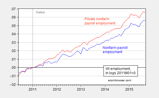
Figure 1: Wisconsin nonfarm payroll employment (blue) and private nonfarm payroll employment (red), s.a., in logs normalized 2011M01=0. Source: BLS and author’s calculations.

As noted elsewhere, Wisconsin employment growth lags that of the US (and neighbor Minnesota).

The Governor cites unemployment rates; he omits the fact that Wisconsin unemployment rates throughout the period for which data are available are typically lower than that in the US overall — about 0.77 percentage points. Figure 2 shows the US minus WI unemployment rate differential, with the 1976M01-2010M12 average in orange.

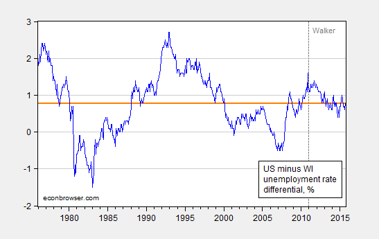
Figure 2: US minus WI unemployment rate, s.a., in % (blue) and 1976M01-2010M12 average (orange bold line). Source: BLS and author’s calculations.

Not only is Wisconsin’s unemployment performance exactly where one would expect on average, over the Governor’s tenure, the US has improved more rapidly than Wisconsin, in terms of unemployment!

Finally, mass layoffs are rising. Figure 3 depicts numbers reported through October 16th of each year, and those numbers normalized by nonfarm payroll employment in September of each year (October figures for 2015 not yet available).

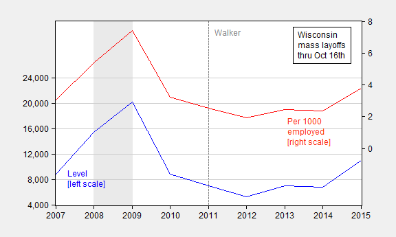
Figure 3: Mass layoffs, reported through October 16th of each year (blue, left scale), and per 1000 nonfarm payroll employed (red, right scale). NBER defined recession dates shaded gray. Source: DWD, BLS, NBER and author’s calculations.

I let the reader decide whether Wisconsin is “moving in the right direction”.

“Collapse and Revival : Understanding Global Recessions and Recoveries”

That’s the title of a new book by Ayhan Kose and Marco Terrones, just released.

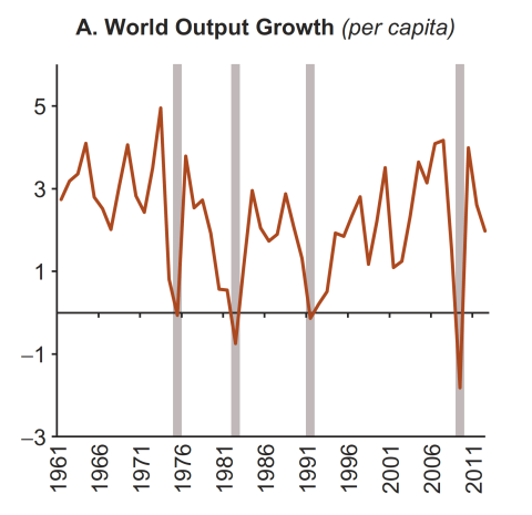
Figure 4.3.A from Kose and Terrones (2015).

Here’s a brief description of the book’s topic.

The world is still recovering from the most recent global recession associated with the 2008-2009 financial crisis, and the possibility of another downturn persists as the global economy struggles to regain lost ground. But what is a global recession? What does it mean to have a global recovery? What really happens during these episodes? As the debates about the recent global recession and the subsequent recovery have clearly shown, our understanding of these questions has been very limited.

This impressive work culminates a research program of central importance—the investigation of the definition and nature of global recessions and recoveries. The authors deploy a comprehensive statistical documentation of global business cycles in an accessible—yet empirically rigorous—fashion, weaving in the most recent thinking on the linkages between financial crises, recessions and recoveries. In my view, this volume is sure to become the standard reference on this important subject. IMF Chief Economist Maury Obstfeld, as well as Ken Rogoff, Mark Watson, Eswar Prasad and Michael Bordo make similar assessments.

Assessing the Counter-cyclical Macro Policies of the Great Recession

There are at least two ways of proceeding. One could repeat the following mantra endlessly:

[T]he government taxes or borrows the resources used to build infrastructure projects. Government spending crowds resources out from the rest of the economy. More federal spending comes at the expense of a smaller private sector.

These factors explain why the 2009 stimulus failed. So did Japan’s decade-long attempt to stimulate its economy through infrastructure projects. The Japanese wound up with massive debt, superhighways in underpopulated rural districts—and an anemic economy.

As far as I know, this 2014 statement from the Heritage Foundation is not based on a given econometric study, but is an article of faith, much like the assertion of “The Treasury View” discussed in this post.

Or, one can appeal to extant estimates of multipliers to estimate how the economy would have performed in the absence of fiscal and monetary stimulus and financial system rescuses. That is exactly what is done in a Blinder-Zandi CBPP study, with the results shown in Figure 1.

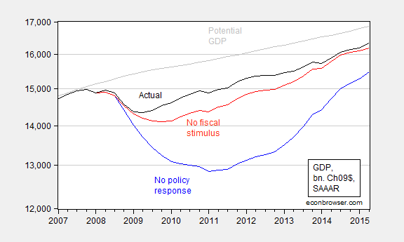
Figure 1: Actual GDP (black), counterfactual GDP under no economic response (blue), counterfactual GDP under no fiscal response (red), potential GDP (gray bold), all in billions Ch.2009$, SAAR; log scale. Source: Blinder and Zandi (2015), appendix tables B1, B2; and CBO, Budget and Economic Outlook (August 2015), via FRED.

The fiscal policies include not just the ARRA (discussed here and here) but also the Economic Stimulus Act of 2008, implemented under G.W. Bush, extended unemployment insurance benefits, and payroll tax relief. Of the total 1,484 billion outlays, slightly under half took the form of tax cuts ($701 billion) and slightly over half in spending ($783 billion).

Links for 2015-10-18

Quick links to a few items I found interesting.

From the Economic Review of the Federal Reserve Bank of Kansas City:

We find oil-specific demand shocks largely drove the oil price movements since mid-2014, reflecting shifts in expectations about future supply relative to future demand. In particular, the driving factors behind the decline appear to be expectations that the future supply of oil will remain higher, or at least more stable, and concerns about weakening future demand due to slowing global growth forecasts.

From a new study by James Feyrer, Erin Mansur, and Bruce Sacerdote:

The combining of horizontal drilling and hydrofracturing unleashed a boom in oil and natural gas production in the US. This technological shift interacts with local geology to create an exogenous shock to county income and employment. We measure the effects of these shocks within the county where production occurs and track their geographic propagation. Every million dollars of oil and gas extracted produces $66,000 in wage income, $61,000 in royalty payments, and 0.78 jobs within the county. Outside the immediate county but within the region, the economic impacts are over three times larger. Within 100 miles of the new production, one million dollars generates $243,000 in wages, $117,000 in royalties, and 2.49 jobs. Thus, over a third of the fracking revenue stays within the regional economy. Our results suggest new oil and gas extraction led to an increase in aggregate US employment of 725,000 and a 0.5 percent decrease in the unemployment rate during the Great Recession.

And from the always insightful Bill McBride:

Here is a review of three key demographic points:

Demographics have been favorable for apartments, and will become more favorable for homeownership.
Demographics are the key reason the Labor Participation Rate has declined.
Demographics are a key reason real GDP growth is closer to 2% than 4%.

Guest Contribution: “Migration, “Free” Trade and China in History”

Today we are fortunate to have a guest contribution by Robert J. Schwendinger, former Executive Director of the Maritime Humanities Center of the San Francisco Bay Region, and author of the newly republished volume Ocean of Bitter Dreams: The Chinese Migration to the United States, 1850-1915 (Long River Press).

In my work, Ocean of Bitter Dreams, I document the workings of imperialist economics for a critical era in trans-Pacific relations. Those nationals in China — the British, French, Spanish, Dutch, Prussians, and many Americans — preyed on vulnerable Chinese during the formative years, and reaped unimaginable fortunes for that time.

Opium and “Free” Trade

My book traces the actions of Americans who participated in the Opium Wars, the “coolie” trade — essentially a parallel slave trade — and the treatment of immigrating Chinese to the United States. Their attitudes are bound irrevocably to the exclusion of Chinese well into the 20th Century.

Opium was a prime merchandise of the age. By the time the Emperor directed Prince Kung to move against the illegal importation along the coast, the complex network was virtually impregnable. The Imperial Navy was a ghost of its former self, suffering from measures taken in the Fifteenth Century to reduce the high costs of a grand navy. Existing vessels were few, slow, and ineffective.

Interests as far as half a globe away depended on the illicit opium. Bengal received over half its revenues from the cultivation and sales, as traders, shippers, captains, bankers in England, the United States, and Portugal, reaped ever increasing profits from its distribution. American’s share of the drug was approximately twenty-percent, taking the lion’s share from Turkey. Leading American traders such as Samuel Russell and Company were part of an interlocking, mutually supporting network that included among other New Englanders, John P. Cushing, John Jacob Astor, and the Perkins brothers.

Prince Kung, a key statesman in the late Ching dynasty, attempted to put a halt to the traffic in 1839. He appointed Commissioner Lin Tse-Hsu to carry out a firm policy against the opium trade. Lin wrote Queen Victoria, and asked why she was forcing opium on the Chinese even as she forbade her own people to smoke the drug. He asked if there was no end to Britain’s desire for profit. After receiving an unsatisfactory reply, Lin set out to destroy 20,283 chests of opium that were confiscated from foreign factories at Canton, eight floating depots, and coastwise clippers. The 3,564 pounds of “black dirt,” worth about ten million dollars at that time, was pulverized on platforms suspended across huge trenches, then laborers stirred the residue in water, salt, and lime. Boiling from the volatile mixture, the trenches looked like great scalding furnaces; the stench was overwhelming in the intense heat of the Canton Delta. It took two months to collect the valuable contraband and thee weeks to dispose of it. In anticipation of the wholesale destruction, Commissioner Lin prayed to the God of the Sea, appealing to all sea creatures to seek safe harbors until the “poison” dispersed throughout the seas.

Shortly after the destruction of opium, England sent the largest expeditionary force ever witnessed in Chinese waters. The first Opium War led to another in 1856, then in 1860 British and French troops destroyed the magnificent and singular treasure house of China, the incredible Summer Palace outside Peking. Palace grounds included forest, gardens, man-made lakes, bridges, and a compound of two hundred buildings, many roofed with gold. They were filled with the finest silks, jade, gold ornaments, rare art, and irreplaceable libraries. In a highly symbolic act, comparable to the sack of Rome by the barbarians, those armies looted and reduced to ruins what took centuries of Chinese culture to produce.

After approximately eleven years of hostilities, gunboat diplomacy wrested over fifty million dollars in indemnities; ceded the island of Hong Kong to Britain, including the New territories, 376 miles of mainland, islands and bays; and granted extra-territoriality rights to the allied powers.

The agreements that grew out of China’s bitter experience have been described as the “unequal treaties.” Eventually all Western shipping was freed from Chinese control in her own waters. The five Treaty Ports that were granted after the first Opium War eventually grew to eighty by the end of hostilities. Missionaries were accorded freedom to proselytize anywhere, and opium was blessed with legal status, becoming the prime merchandise of the age. Imports increased over three hundred percent in ten years.

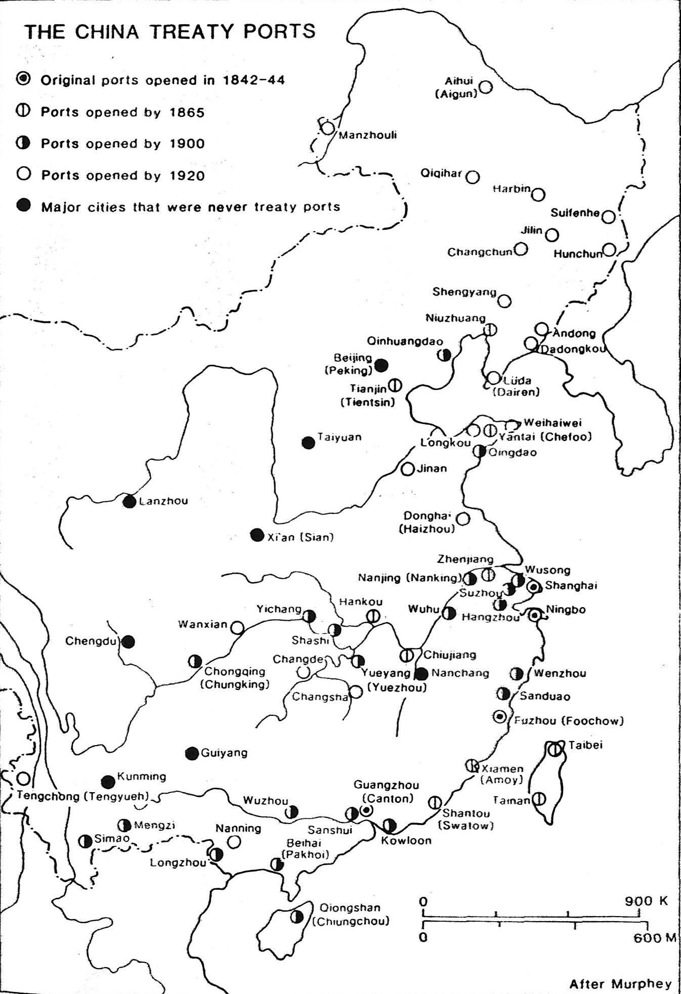
Figure 1: Five Treaty ports were opened to foreign trade in 1842 as a result of the first Opium War: Canton, Amoy, Foochow, Ningpo, and Shanghai. The number eventually grew to more than eighty. The Liu-chiu Islands, or Lew Chu, is currently the Ryukyu Archipelago.

The “Coolie Trade”

The unequal treaties drove China into a position of astonishing vulnerability. The infamous “Coolie Trade” would not have been possible without the opening of all those treaty ports and the granting of those extraordinary rights.

Hong Kong was an economic and symbolic prize. It depended on the distribution of opium, the increase of Chinese residents, a large percentage of import/exports between China and other countries, the emigration movement, and the manufacturing of chains and other restraints that were used in the “Coolie” trade.

While African slaves were being freed in the United Kingdom and South America, the “Coolie Trade” grew out of the desire to supplement or replace the slaves. The term “Coolie,” became the derogatory designation for cheap, mostly servile labor.

The discovery of gold in California attracted Chinese as immigrants, as were populations in other parts of the world. There grew out of the movement those Chinese who were considered “free” emigrants, who were able to pay for their tickets to the United States, as distinguished from “coolie” immigrants, in the belief that the ability to pay for the voyage was a qualitative difference between the two. Those without the ability to pay and entrusted themselves to contractors or were deceived into shipping out, were sent to the Sandwich Islands, Mauritius, Panama, Peru, Brazil, and the West Indies. They were looked upon as “coolie” and maligned with a host of descriptions, from “voluntary slaves” to a “degraded class of semi-barbarians.”

As attractive were the rewards from opium for British, French, Portuguese, and Americans, especially, the rewards for recruiting unsuspecting Chinese men and boys were just as high. Shippers and captains depended on unscrupulous brokers to entice Chinese to the ports, as they were either lied to, kidnapped, or duped into signing false labor contracts.

In some ports, far from the arm of Chinese law, barracoons, not unlike those that dotted the African coast, were erected to hold the vulnerable males and they were monitored by armed guards. Approximately three-quarters of a million men and boys ended up in the “coolie” trade.

Richard Henry Dana, author of Two Years Before the Mast, while in Cuba, witnessed the selling of males in the marketplace. He wrote that the price paid for a Chinese laborer was $400.00.

The sailings of American vessels, carrying from 244 to 500 souls each, were plagued with disastrous events. Many Chinese rebelled against their captors. Numerous Chinese died from being fired on or kept secured in the hold of ships and suffocated. Many became lost in tumultuous weather, and untold numbers died before they could outlive their service. The case of the Robert Bowne, the most documented “coolie” ship and throughly developed in this book, provides particular insight into the deadly trade.

America’s Role

In my studies, I identified thirty one American vessels involved in the trade. Many of them were famous clipper ships of the period, Swordfish, Sea Witch, Winged Racer, and Live Yankee. In addition, there are at least 116 more American ships under sail that were tallied by a port official in Cuba. Add to that incredible number those vessels that brought human cargoes to the Chincha Islands of Peru, Brazil, Panama, Mauritius, and others. As the trade became more disreputable, Western nations gradually withdrew, and the Americans who participated became major transporters.

Even then, my tabulation of the ships involved is assuredly incomplete. The ocean can never reveal its dead: those ships that shipwrecked, those Chinese who rebelled and were killed, those vessels that had registered false names at ports of arrival, those captives who committed suicide where they labored or became sick and useless on board and were thrown into the sea, the vessels that ship owners managed to keep out of Lloyd’s Register of Ships, and those Chinese who would never grace a ship’s passenger list, or have a death certificate signed for them, nor would so many be remembered for their presence, trapped forever in that malevolent trade, would never be known.

“Coolie” activity commanded profits that were staggering for the time: an approximate $300 million was earned overall; the Americans share was an approximate $140 million or the 1988 equivalent of approximately $1.5 billion [or 2014 equivalent of about $3 billion, using the CPI to adjust]. The number of American voyages more than likely approximated 900 over the period, requiring a remarkable movement of vessels for any time.

The ships under sail transporting Chinese immigrants to California in particular, loaded their human cargoes with little concern for the comfort of their passengers. Charging as much as the passage would allow, ship owners earned unprecedented fortunes. The same conduct carried over into the transportation on board the great transpacific steamships that began to monopolize the route between China and the United States. The two foremost steamship lines were the Pacific Mail and the Occidental and Oriental, registered as California corporations.

American politicians, unions, and newspapers, particularly in the West, concentrated their scorn on what they considered an inseparable triad: the “China ships,” as the transpacific steamships were called, the Chinese passengers who traveled in them, and the Chinese crews that manned them. Immigrant, ship, and sailor bore the bitter attacks of slander and hatred.

Antipathy toward Chinese culminated in the passage of the Chinese Exclusion Act of 1882. Tightened restrictions of the Act continued well into the 20th Century.

Concluding Thoughts

The seeds of failure for a prosperous China Trade were being planted during the years in which western nations treated China as a semi-colony, taking as much as they could get and giving little or nothing in return. The failure was also precipitated by the nations in which Chinese nationals were exploited for their labor, but denied universal rights and protections.

The story of Commissioner Lin Tse Hsu and his destruction of the great quantity of opium in 1839 is as important to Chinese history as the Boston Tea Party is to the United States; and although Lin’s actions precipitated defeat by the Western powers, the national humiliation China and Chinese suffered for almost a century is partly responsible for the two revolutions in modern times. With an emphasis on its own needs, China will assuredly measure each petitioner for respect. That nation’s history also suggests the need to be especially aware of challenges to its sovereignty.

This post written by Robert J. Schwendinger.

Economic effects of shocks to oil supply and demand

How can we estimate the separate economic effects of shocks to oil supply and demand? I’ve just finished a research paper with Notre Dame Professor Christiane Baumeister that develops a new approach to this question.



The basic reason the question is hard to answer is that we would need to know the value of two key parameters: the response to price of the quantity supplied (summarized by the supply elasticity) and the response to price of the quantity demanded (summarized by the demand elasticity). If we only observe one number from the data (the correlation between price and quantity), we can’t estimate both parameters, and can’t say how much of observed movements come from supply shocks and how much from demand.

One way to resolve this problem is to find another observed variable that affects supply but not demand. A generalization of this idea is the basic principle behind what is referred to as structural vector autoregressions, in which we might also exploit information about the timing of different responses. The simplest version of this would be an assumption that it takes longer than one month for supply to respond to changes in price. If the very short-run supply elasticity is zero, and if supply shocks are uncorrelated with demand shocks, then the correlation between the error we’d make in forecasting quantity and price one month ahead could be interpreted as resulting from the very short-run response of demand to price. Putting this together with the observed dynamic correlations between the variables (for example, the correlation between this month’s quantity and last month’s price) would allow us to identify the effects of the different shocks over time.

In a previous paper that will be published in the September issue of Econometrica, Christiane and I proposed that Bayesian methods could allow us to generalize the traditional approach to structural vector autoregressions. We noted that what is usually treated as an identifying assumption (for example, the restriction that there is zero response of supply to the unexpected component of this month’s change in price) could more generally be represented as a Bayesian prior belief– we may believe it’s unlikely there is a big immediate response of supply to price but should not rule the possibility out altogether. Our paper showed how one can perform Bayesian inference in general vector dynamic systems where there may be good prior information about some of the relations but much weaker information about others.

In our new paper Christiane and I apply this method to study the role of shocks to oil supply and demand. We begin by reproducing an influential investigation of this question by University of Michigan Professor Lutz Kilian that was published in American Economic Review in 2009. Kilian studied a 3-variable system based on oil production, price and a measure of global economic activity. He assumed that supply does not respond contemporaneously to price or economic activity and that economic activity does not respond contemporaneously to oil production, assumptions that are referred to as the Cholesky approach to identification.

We first reproduced Kilian’s results using his dataset and his methodology. The panels below summarize the effects of three different kind of shocks (represented by different rows) on each of the three variables (represented by different columns). The horizontal axis in each panel is the number of months since the shock first hits at date 0. The red lines are the estimates that Kilian came up with based on his Cholesky identification.

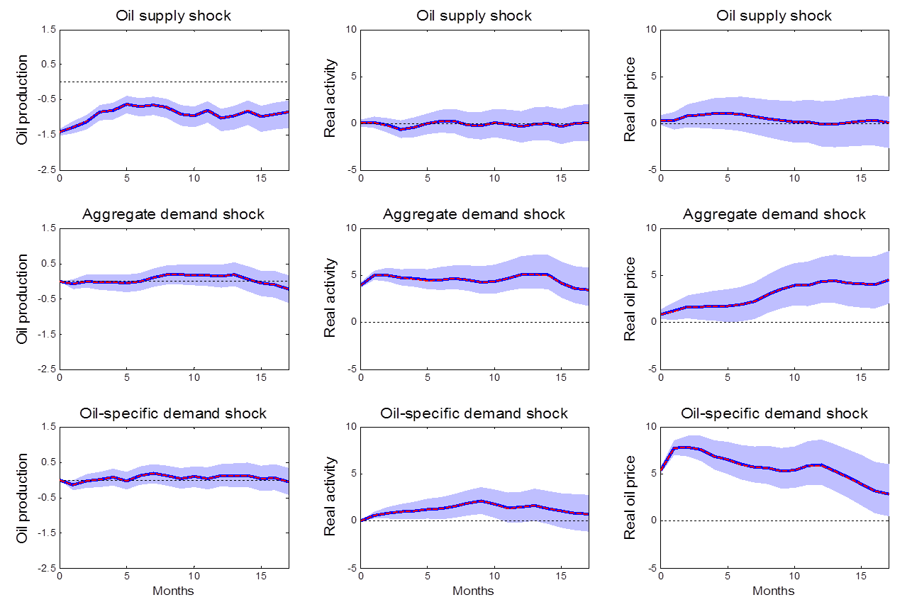
Effects of 3 different shocks on 3 different variables as estimated using the Kilian (2009) Cholesky identification. Red lines give Kilian’s original estimates. Blue lines and shaded regions give posterior medians and 95% posterior credibility sets when the approach is implemented as a special case of Bayesian inference. Source: Baumeister and Hamilton (2015).

We then formulated the same approach as a special case of Bayesian inference, in which we have dogmatic prior beliefs about the contemporaneous response of supply to price and economic activity but very uninformative prior information about the contemporaneous response of demand to price and economic activity. We conducted this Bayesian inference as a special case of the algorithms developed in our Econometrica paper. Incidentally, anybody can download the MATLAB code to do this kind of exercise themselves from my webpage. The Bayesian posterior median and 95% posterior credibility sets are indicated in blue. Not surprisingly, these are exactly the same answer as Kilian obtained using the traditional method.

Is there any benefit to reframing the traditional approach as a special case of Bayesian inference? One of the natural byproducts of our algorithm is the Bayesian posterior inference (that is, what we believe now that we have seen the data) about magnitudes such as the short-run demand elasticity of oil. It turns out that if we had the Bayesian prior beliefs that are implicit in Kilian’s approach, now that we have seen the data, we would still insist that the short-run supply response is zero (because our Bayesian prior beliefs about this parameter were dogmatic), but we would now also be very confident that the short-run demand elasticity is greater than two in absolute value and readily believe that it might be minus or plus infinity. In other words, we do not regard it as the least implausible to conclude that within a month of a 1% increase in oil price, in response consumers might increase their consumption of oil by a million percent or more. Quoting from our paper:

The claim that we know for certain that supply has no response to price at all within a month, and yet have no reason to doubt that the response of demand could easily be plus or minus infinity is hardly the place we would have started if we had catalogued from first principles what we expected to find and how surprised we would be at various outcomes. The only reason that thousands of previous researchers have done exactly this kind of thing is that the traditional approach required us to choose some parameters whose values we pretend to know for certain while acting as if we know nothing at all about plausible values for others. Scholars have unfortunately been trained to believe that such a dichotomization is the only way that one could approach these matters scientifically.

Misgivings about the traditional method are one reason that many researchers have looked for other approaches to identification, such as relying on sign restrictions– surely we can at least rule out that consumers increase the quantity they buy when the price goes up. In a subsequent paper with University of Virginia Professor Daniel Murphy, Kilian used sign restrictions to achieve partial identification and replaced the assumption that there is no contemporaneous response of supply with a hard upper bound on the size of the contemporaneous response. My paper with Christiane shows that the Kilian-Murphy results can also be obtained as a special case of Bayesian inference. We note among other concerns that their specification still allows for an implausibly large contemporaneous response of demand, ignores a good deal of other informative prior information, and yet is still dogmatic about other magnitudes that we really do not know for certain.

The main point of our paper is that if researchers had thought about what they were doing as a Bayesian exercise from the very beginning, there is a much richer set of prior information that could be drawn on while simultaneously relaxing many of the dogmatic restrictions. We illustrate how this can be done for the question of the role of oil supply and demand shocks in particular. Among other contributions, as in a later paper by Kilian and Murphy (2014) we bring inventories into the analysis (as a key reason why quantity and price need not move together), allow for measurement error in the variables (a ubiquitous problem in macroeconomics that is usually entirely ignored in most research), allow the possibility that the relations have changed over time (with the Bayesian approach offering a middle ground between assuming on the one hand that all the data are equally useful or throwing out earlier data altogether on the other), and make use of detailed evidence from other datasets about the price and income elasticities of supply and demand.

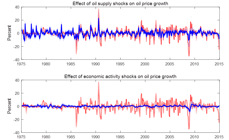
The figure below presents a few of the results we come up with. These are dynamic responses (like those in the first figure above) of global industrial production (the first column) and the real oil price (the second column) to each of the four shocks we study (shocks to supply, economic activity, oil consumption demand, and inventory demand). All four shocks would raise the price of oil, as seen in the second column. But whereas an oil price increase that results from a supply reduction leads to a decline in economic activity, the same is not true of an oil price increase that results from an increase in demand.

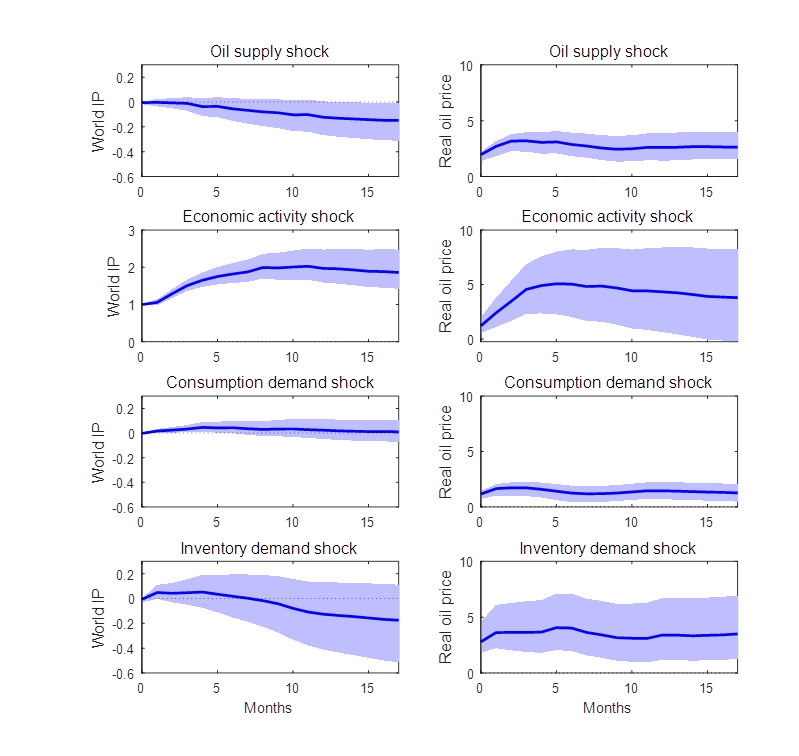
Effects of 4 different shocks on 2 different variables as estimated using the general Bayesian approach in Baumeister and Hamilton (2015). Blue lines and shaded regions represent posterior medians and 95% posterior credibility sets.

Another thing we do in the paper is look at the contribution of different shocks to historical movements in each of the variables. The red lines in each of the 4 panels below plot the actual percent change in the crude oil price each month over 1975-2014. The blue lines give the Bayesian posterior estimate of how big the percent change that month would have been if there had been only one shock. For example, the first panel isolates the contribution of supply shocks. Ninety-five percent posterior credibility regions for the estimates are indicated by light blue shaded regions.

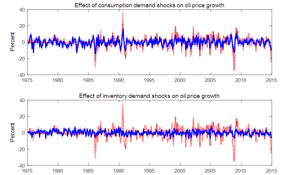
Red lines: actual monthly percent change in refiner acquisition cost for crude petroleum, 1975-2014. Blue lines and shaded regions: estimated contribution of indicated shock. Source: Baumeister and Hamilton (2015).

Again quoting from the paper:

Supply shocks were the biggest factor in the oil price spike in 1990, whereas demand was more important in the price run-up in the first half of 2008. All four structural shocks contributed to the oil price drop in 2008:H2 and rebound in 2009, but apart from this episode, economic activity shocks and speculative demand shocks were usually not a big factor in oil price movements. Interestingly, demand is judged to be a little more important than supply in the price collapse of 2014:H2.

We have drawn on a lot of prior information in producing the above graphs, though none of that information was used dogmatically as has been the case in previous studies. Another advantage of our approach is that we can examine what happens if we had considerably less confidence in any elements of the maintained prior beliefs. The last section of our paper explores the sensitivity of our main conclusions to such changes. We find that although our posterior credibility sets for most objects of interest would be wider when we have less faith in any specified components of the Bayesian prior, most of our broad conclusions would still emerge. For example, we did not find any specification for which there is more than a 2.5% posterior probability that supply shocks accounted for more than 2/3 of the cumulative oil price decline in the second half of 2014.

Our paper concludes:

Prior information has played a key role in every structural analysis of vector autoregressions that has ever been done. Typically prior information has been treated as “all or nothing”, which from a Bayesian perspective would be described as either dogmatic priors (details that the analyst claims to know with certainty before seeing the data) or completely uninformative priors. In this paper we noted that there is vast middle ground between these two extremes. We advocate that analysts should both relax the dogmatic priors, acknowledging that we have some uncertainty about the identifying assumptions themselves, and strengthen the uninformative priors, drawing on whatever information may be known outside of the dataset being analyzed.

We illustrated these concepts by revisiting the role of supply and demand shocks in oil markets. We demonstrated how previous studies can be viewed as a special case of Bayesian inference and proposed a generalization that draws on a rich set of prior information beyond the data being analyzed while simultaneously relaxing some of the dogmatic priors implicit in traditional identification. Notwithstanding, we end up confirming many of the conclusions of earlier studies. We find that oil price increases that result from supply shocks lead to a reduction in economic activity after a significant lag, whereas price increases that result from increases in oil consumption demand do not have a significant effect on economic activity. We also examined the sensitivity of our results to the priors used, and found that many of the key conclusions change very little when substantially less weight is placed on various components of the prior.

To what problem is this legislation a solution to?

People with concealed weapon licenses would be allowed to carry guns inside the buildings and classrooms of Wisconsin’s public universities and colleges under a bill introduced Monday by two state legislators.

According to the Wisconsin State Journal article, the bills sponsors argue that if only students were armed to the teeth, any gunmen would be quickly taken down.

This is a common view, which to my knowledge has no statistical basis. All we have are anecdotes. See for instance Econbrowser reader Rick Stryker’s argument. In the wake of the Newtown massacre, and in response to a reader’s plea after the Newtown massacre in 2012:

“I want my kid to grow up in a world where owning a shiny piece of metal that can instantaneously end human life with little effort is not normal, or something to be proud of, in the modern world.”

Mr. Stryker provided a further suggestion:

I would agree and so Holiday season I’d like to suggest something that you can put under the Christmas tree: a junior membership in the NRA. It’s only $15 and includes a subscription to Insight magazine. The junior memberships are great ways to teach kids about the proper, legal use of firearms and the importance of gun safety.

Sure. To quote “Yeah, that’s the ticket!”

I’ll appeal instead to data. Here is an interesting correlation, involving actual data. First consider the number of casualties in mass shootings.

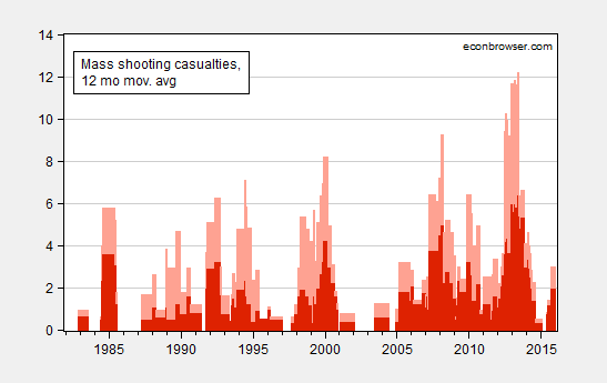
Figure 1: 12 month moving average of mass shooting casualties; deaths (dark red), wounded (pink). Source: Mother Jones, and author’s calculations.

There seems to be a trend…I estimate a tobit model on quarterly data 1982Q1-2012Q4 (since casualties are bounded below at zero):

casualties = -0.376 – 0.989yt-8 + 0.0008timet

Where casualties per million population, y is the output gap expressed as a ratio, and time is a time trend; bold figures denote statistical significance at the 10% level using Huber-White standard errors. The idea is that lagged economic distress induces more attacks. All coefficients are statistically significant, and the standard error of regression is 0.054,

Note the time trend is statistically significant. What is the time trend capturing? I substitute a meaningful variable for the time trend, namely the stock of guns in the US.

casualties = -0.211 – 0.900yt-8 + 0.0006gt

The stock of guns, g, is interpolated from annual data). The standard error of regresion is again 0.054.

This is merely a reflection of a stylized fact about gun violence. For verification of this proposition, see this article (which also contains other data-based observations).

The observation that stricter gun control laws are associated with lower gun violence is suggestive of a constructive — and realistic — path for policy going forward:

Source: Wonkblog.

and not adolescent fantasies about armed citizens policing our campuses. (I must say that if one is worried about “grade inflation”, having hundreds of armed students in classrooms is unlikely to help…)

Guest Contribution: “TPP Critics’ Nighttime Fears Fade by Light of Day”

Today we are fortunate to have a guest contribution written by Jeffrey Frankel, Harpel Professor of Capital Formation and Growth at Harvard University, and former Member of the Council of Economic Advisers, 1997-99. A shorter version appeared at Project Syndicate.

The text of the TPP (Trans Pacific Partnership) that was finally agreed among trade negotiators of 12 Pacific countries on October 5 came as a triumph over long odds. Tremendous political obstacles, domestic and international, had to be overcome over the last five years. Now each country has to decide whether to ratify the agreement.

Many of the issues are commonly framed as “Left” versus “Right” in US politics. The unremitting hostility to the negotiations up until now from the Left – often in protest at being kept in the dark regarding the text of the agreement — has carried two dangers. One danger was that opponents would succeed in blocking negotiations altogether. Indeed, when Democrats in Congress voted against giving President Obama the necessary authority in June, the entire negotiations were widely declared to be dead. This would have been a shame — at least in the view of most economists — because the resulting trade liberalization was very likely in the end to turn out beneficial overall.

The second danger was that the Administration would be forced at the margin to move to the “Right” in order to pick up votes from Congressmen who said they would support the outcome if (and only if) it contained provisions that were sufficiently generous to American corporations. Those concerned about labor and the environment risked hurting their own cause by seeming to say that they would oppose the agreement no matter how well it did at including provisions to their liking, which could have undermined the White House incentive to pursue their issues.

In this light, this month’s outcome is a pleasant surprise. In the first place, the agreement gives the pharmaceutical firms, tobacco companies, and other corporations substantially less than they had asked for — so much so that Senator Orrin Hatch (Utah) and some other Republicans now threaten to oppose ratification in the final up-or-down vote. In the second place, the agreement gives the environmentalists more than most of them had bothered to ask for. I don’t know the extent to which these outcomes were the result of hard bargaining by other trading partners such as Australia. Regardless, it is a good outcome. The domestic critics might consider now taking a fresh look with an open mind.

The issues that are the most controversial in the US are sometimes classified as “deep integration,” because they go beyond the traditional negotiated liberalization in trade tariffs and quotas. Two categories are of positive interest to the Left: labor and the environment. Two categories are of “negative interest” to the Left in the sense that it has feared excessive benefits for corporations: protection of the intellectual property of pharmaceutical and other corporations and mechanisms to settle disputes between investors and states.

Now that the long-delayed agreement is completed, what turns out to be in it? Two good things in the TPP’s environment chapter are especially noteworthy. First, it takes substantial steps to enforce prohibition of trade in endangered wildlife — banned under CITES (Convention on International Trade in Endangered Species) but insufficiently enforced. Second, it also takes substantial steps to limit subsidies for fishing fleets — which in many countries waste taxpayer money in pursuit of the overfishing of our oceans. For the first time, apparently, these environmental measures will be backed up by trade sanctions.

I wish that certain environmental groups had spent half as much time ascertaining the specific possibility of good outcomes like these as they spent in sweeping condemnations of the process. The agreement on fishing subsidies was reached in Maui in July; but critics were too busy to take notice. Fortunately it is not too late for them to climb on board now.

Some NGOs might still worry that these provisions will not be enforced strongly enough. But trade penalties are among the most powerful tools for enforcement of international agreements that exist; for that reason environmental groups in the past have asked that such measures be placed in the service of environmental goals. There is no denying that the TPP provisions on endangered species and fishing are steps forward.

A variety of provisions in the area of labor practices, particularly in Southeast Asia, should also be of interest. They include steps to promote union rights in Vietnam and steps to crack down on human trafficking in Malaysia.

The greatest uncertainties were over the extent to which big US corporations would get what they wanted in the areas of investor-government dispute settlement and intellectual property protection. On the one hand, critics often neglected to acknowledge that international dispute settlement mechanisms could ever serve a valid useful purpose. Similarly, they often neglected to acknowledge that some degree of patent protection is indeed needed if pharmaceutical companies are to have an adequate incentive to invest in research and development of new drugs. But, on the other hand, there was indeed a possible danger that such protections for corporations could have gone too far.

The dispute settlement provisions might have interfered unreasonably with member countries’ anti-smoking campaigns, for example. In the end, the tobacco companies did not get what they had been demanding. Australia is now free to ban brand name logos on cigarette packets. TPP sets a number of other new safeguards against misuse of the investor-state dispute settlement (ISDS) mechanism as well. For example there is a provision for rapid dismissal of frivolous suits. The rest of the details are publically available in clear bullet point form, from USTR, if one takes the trouble to read them.

The intellectual property protections might have extended to other TPP member markets a 12-year period of protection for the data that US pharmaceutical and bio-technology companies compile on new drugs (biologic medical products, in particular), and might have made it too hard for generics to eventually bring the benefits to the public at lower costs. In the end, these companies too did not get much of what they had wanted. The TPP agreement assures protection of their data for only 8 years in some places and 5 years in others and instead relies on the latter countries to use other measures to constrain the appropriation of the firms’ intellectual property.

The focus on new areas of deep integration should not obscure the old-fashioned free-trade benefits that are also part of TPP: reducing thousands of existing tariff and non-tariff barriers that inhibit trade. Many of these reductions benefit US exports. (Most US barriers against imports were already very low.) Liberalization in manufacturing includes the auto industry, for example. Liberalization in services includes the internet.

The liberalization of agriculture is noteworthy; this sector has long been a stubborn holdout in international trade negotiations. Countries like Japan have agreed to let in more sugar, beef, pork, rice and dairy products, from more efficient producer countries like Australia and New Zealand. In all these areas and more, traditional textbook arguments about the gains from trade apply: new export opportunities, higher wages, and a lower cost of living.

Many citizens and politicians made up their minds about TPP some time ago, based on having read seemingly devastating critiques of what was feared would emerge from the trade negotiations. When the text of the agreement is released is the time for the critics to read the specifics that they have so long hungered to see and to decide whether they can support it after all. They just might discover that their nighttime fears are much diminished by the light of day.

This post written by Jeffrey Frankel.

How do consumers respond to lower gasoline prices?

U.S. gasoline prices averaged $3.31 a gallon over December 2013 to February 2014 but only $2.31 a gallon over December 2014 to February 2015. How did consumers respond to this windfall in their spending power? A new study by the JP Morgan Chase Institute has come up with some interesting answers.

Rather than trying to draw conclusions from imperfect aggregate or survey data, the Chase study is based on the anonymized credit or debit card transactions of 25 million individuals over these two periods of high versus low gasoline prices. They found huge differences across individuals in terms of how important gasoline is for their budget. A typical household was spending $101 a month on gasoline back when gas prices were high. For the highest-spending quintile, that number was $359/month, whereas for the lowest quintile it was only $2/month. And spending on gasoline is a much bigger fraction of the budget for lower income households.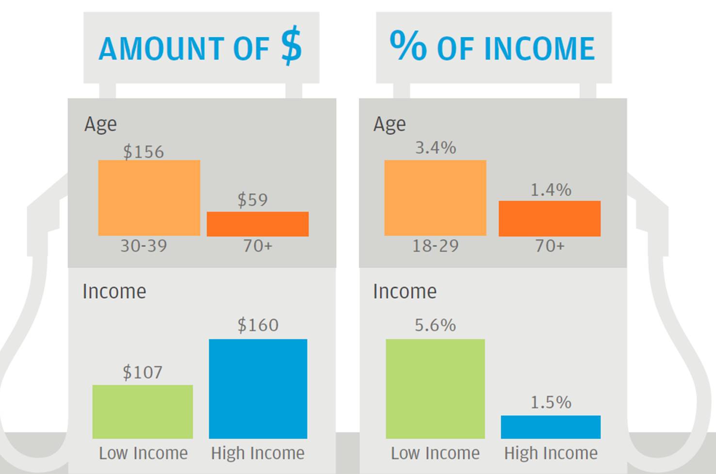

Spending on gasoline by different income quintiles and age groups (total dollars and as a percent of percent of income). Source: JP Morgan Chase Institute.

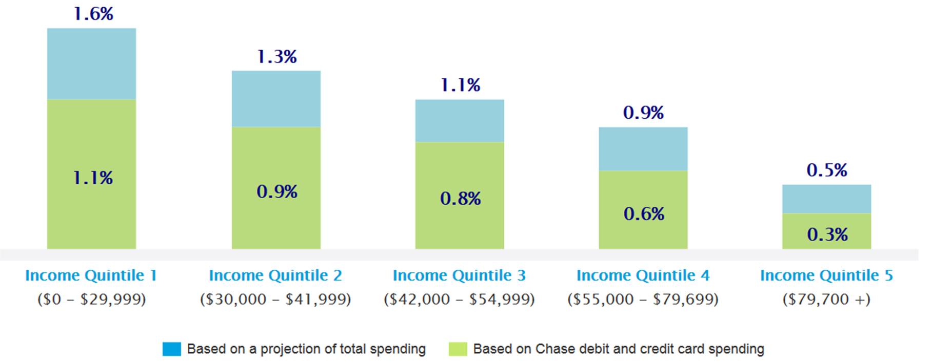
Increase in purchasing power from gasoline saving for different income groups. Source: JP Morgan Chase Institute.

I and others have tried to infer the effects of lower gasoline prices on consumer spending by looking at aggregate consumption spending. But using their detailed data set the Chase researchers were able to come up with a more satisfying answer. The basic idea is to compare how much spending on other items changed between the high gas price and low gas price periods for those who had been spending a large amount on gasoline with those who had been spending a low amount on gasoline. Economists refer to this as inference based on difference in differences. The Chase researchers found 73 cents in extra spending on other items for every dollar saved at the gasoline pump. Restaurants and groceries were the two biggest areas where spending was observed to increase.

Percent of gasoline saving spent on other categories. Source: JP Morgan Chase Institute.

One limitation of the data set is that most car purchases are not done with credit cards. We know from the aggregate data that increased car purchases are a big component of the consumer response to lower gasoline prices. Thus the total extra spending is likely to be significantly higher than the 73% measured directly.

The evidence thus is that consumers were indeed responding to the most recent price declines the same way they usually did, namely, by spending most of the windfall. The fact that we don’t see this as clearly in the aggregate data suggests that the economy has been facing other headwinds that partly offset the stimulus from lower gasoline prices.

Another consumer response to lower gasoline prices is increased consumption of gasoline itself, though these adjustments take more time to develop. U.S. vehicle miles traveled, which had been stagnant while gas prices were high, have since resumed their historical growth.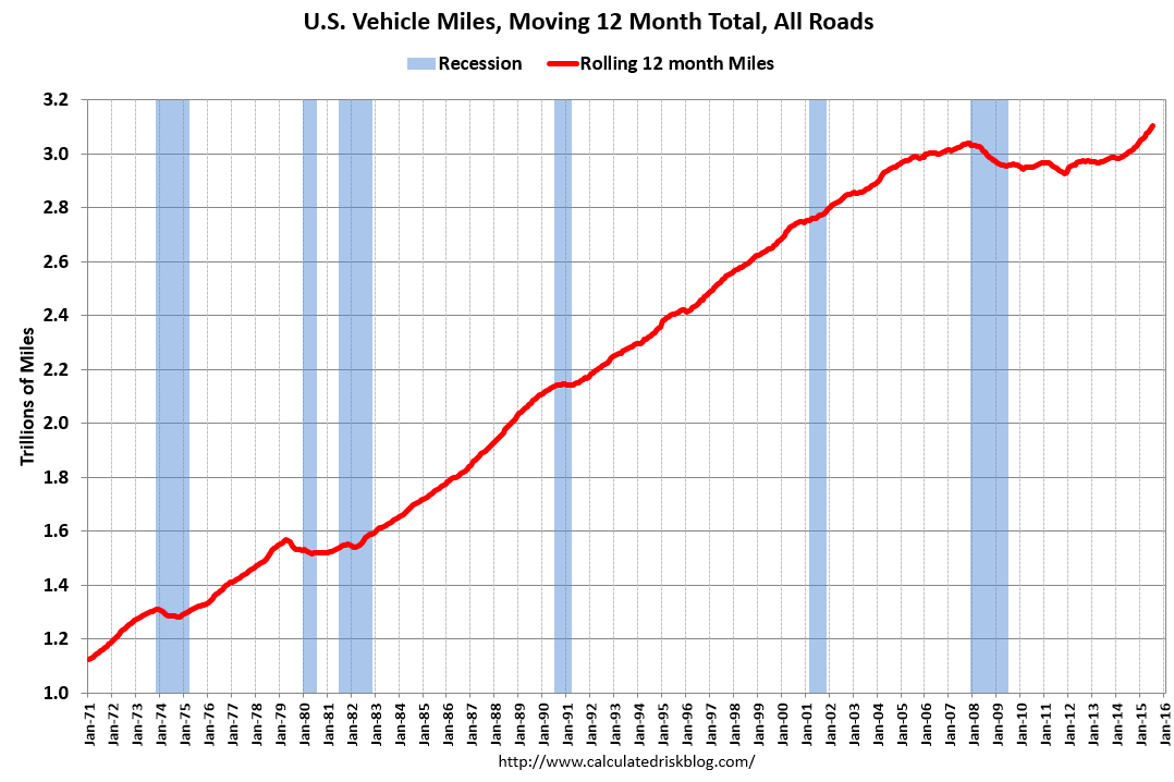

Source: Calculated Risk.

And the average fuel efficiency of new vehicles sold in the United States, which had been improving steadily through most of 2014, has fallen with oil prices.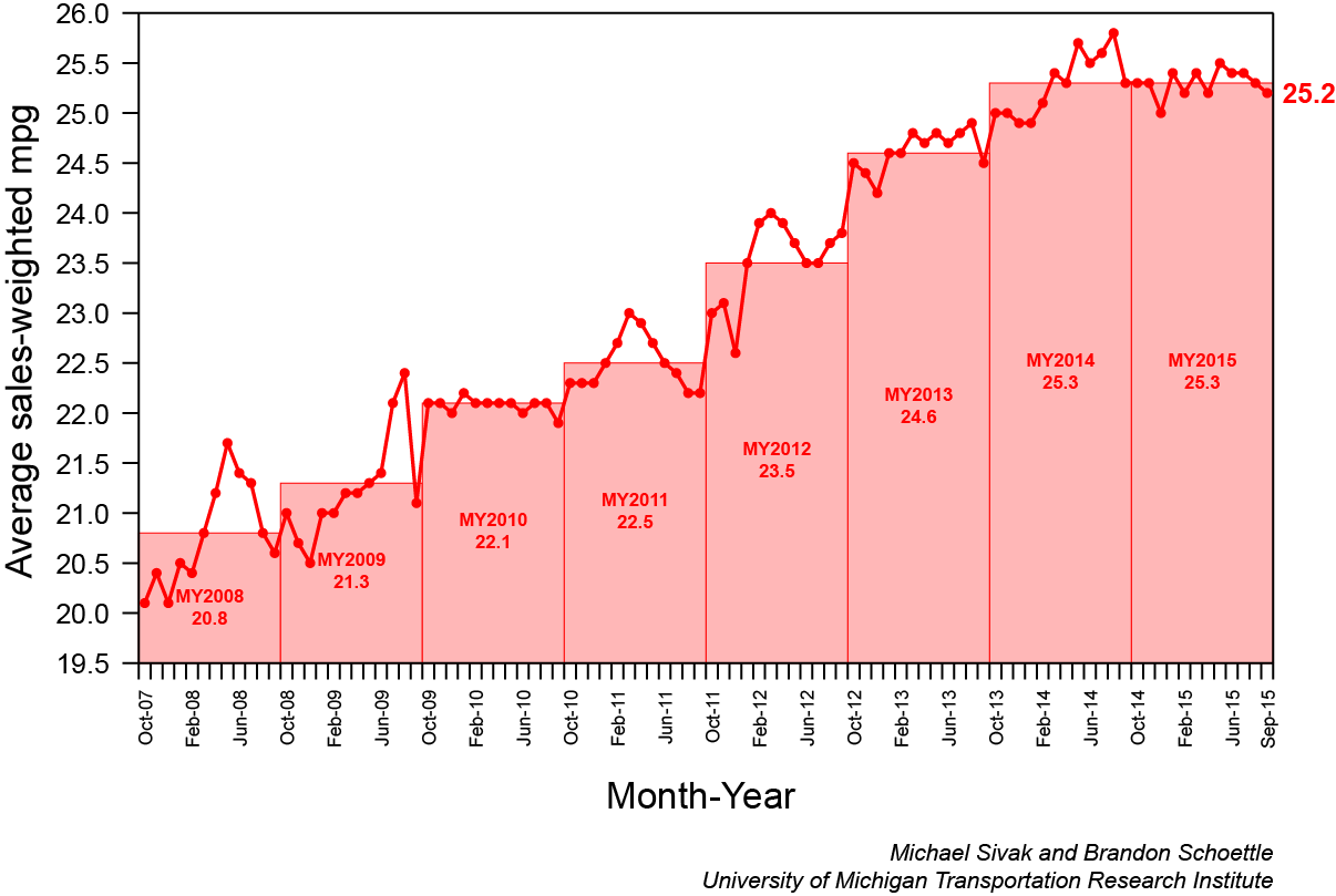

Source: University of Michigan Transportation Research Institute.

Outsourced Monetary Tightening

From Zeng and Wei in the Wall Street Journal today:

Central banks around the world are selling U.S. government bonds at the fastest pace on record, the most dramatic shift in the $12.8 trillion Treasury market since the financial crisis.

The article continues:

many investors say the reversal in central-bank Treasury purchases stands to increase price swings in the long run. It could also pave the way for higher yields when the global economy is on firmer footing, they say.

…

Foreign official net sales of U.S. Treasury debt maturing in at least a year hit $123 billion in the 12 months ended in July, said Torsten Slok, chief international economist at Deutsche Bank Securities, citing Treasury Department data. It was the biggest decline since data started to be collected in 1978. A year earlier, foreign central banks purchased $27 billion of U.S. notes and bonds.

Using estimates in Kitchen and Chinn (2012), we can calculate the increase in yields that have already occurred. Table 1 presents estimates from a regression of ten year yields on the cyclically adjusted budget surplus, Fed purchases and foreign purchases (plus activity variables).

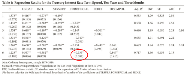
Source: Kitchen and Chinn (2012)

Constraining the slope coefficient on these three variables to be equal (after sign switches), we obtained a point estimate of 0.335 (circled in red).

Potential GDP according to CBO in 2015Q2 was $18425 billion (SAAR). The ratio of net sales to potential GDP is thus is 0.0067 (0.67%) Using our estimate of 0.335, I get an elevated ten year yield of 0.22 percentage points relative to what otherwise would have occurred.

None of this should be too surprising; back in April, I pointed out that foreign exchange reserves (of which 60% of emerging market/LDC holdings are in US dollars) were declining.

For those who are attracted to apocalyptic views (e.g., here), a $1 trillion net sale of Treasurys would result in a 1.82 percentage points increase in yields (0.0543 ratio to potential GDP times 0.335, indicating a 1.82 ppt increase). That being said, there are other downward forces on yields, including deficient aggregate demand (aka secular stagnation).

Nonetheless, the prospects for upward pressure on long term yields (on top of the appreciated dollar) suggests caution in tightening monetary policy.