
Metin Bektas's Blog: Metin's Media and Math
May 2, 2016
World Population – Is Mankind’s Explosive Growth Ending?
According to the World Population Clock there are currently about 7.191 billion people alive. This year there have been 118 million births (or 264 per minute) and 49 million deaths (or 110 per minute), resulting in a net growth of 69 million people. Where will this end? Nobody can say for sure. But what we can be certain about is that the explosive growth has been slowing down for the past 40 years. I’ll let the graphs tell the story.
Here is how the world population has developed since the year 1700. The numbers come from the United Nations Department of Economic and Social Affairs. From looking at the graph, no slowdown is visible:

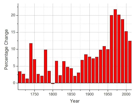
However, another graph reveals that there’s more to the story. I had the computer calculate the percentage changes from one decade to the next. From 1960 to 1970 the world population grew by 22 %. This was the peak so far. After that, the growth rate continuously declined. The percentage change from 2000 to 2010 was “only” 12 %.
Of course it’s too early to conclude that this is the end of mankind’s explosive growth. There have been longer periods of slowing growth before (see around 1750 and 1850). But the data does raise this question.
Talk to me again when it’s 2020 or 2030.
Just by the way: according to estimates, about 108 billion people have been born since the beginning of mankind (see here). This implies that about 101 billion people have died so far and that of all those born, 6.5 % percent are alive today.
Did somebody say dust in the wind?
Here is how the world population has developed since the year 1700. The numbers come from the United Nations Department of Economic and Social Affairs. From looking at the graph, no slowdown is visible:
However, another graph reveals that there’s more to the story. I had the computer calculate the percentage changes from one decade to the next. From 1960 to 1970 the world population grew by 22 %. This was the peak so far. After that, the growth rate continuously declined. The percentage change from 2000 to 2010 was “only” 12 %.
Of course it’s too early to conclude that this is the end of mankind’s explosive growth. There have been longer periods of slowing growth before (see around 1750 and 1850). But the data does raise this question.
Talk to me again when it’s 2020 or 2030.
Just by the way: according to estimates, about 108 billion people have been born since the beginning of mankind (see here). This implies that about 101 billion people have died so far and that of all those born, 6.5 % percent are alive today.
Did somebody say dust in the wind?


Inflation: How long does it take for prices to double?
A question that often comes up is how long it would take for prices to double if the rate of inflation remained constant. It also helps to turn an abstract percentage number into a value that is easier to grasp and interpret. If we start at a certain value for the consumer price index CPI0 and apply a constant annual inflation factor f (which is just the annual inflation rate expressed in decimals plus one), the CPI would grow exponentially according to this formula:
CPIn = CPI0 · f^n
where CPIn symbolizes the Consumer Price Index for year n. The prices have doubled when CPIn equals 2 · CPI0. So we get:
2 · CPI0 = CPI0 · f^n
Or, after solving this equation for n:
n = ln(2) / ln(f)
with ln being the natural logarithm. Using this formula, we can calculate how many years it would take for prices to double given a constant inflation rate (and thus inflation factor). Let’s look at some examples.
——————–
In 1918, the end of World War I and the beginning of the Spanish Flu, the inflation rate in the US rose to a frightening r = 0.204 = 20.4 %. The corresponding inflation factor is f = 1.204. How long would it take for prices to double if it remained constant?
Applying the formula, we get:
n = ln(2) / ln(1.204) = ca. 4 years
More typical values for the annual inflation rate are in the region several percent. Let’s see how long it takes for prices to double under normal circumstances. We will use r = 0.025 = 2.5 % for the constant inflation rate.
n = ln(2) / ln(1.025) = ca. 28 years
Which is approximately one generation.
One of the highest inflation rates ever measured occurred during the Hyperinflation in the Weimar Republic, a democratic ancestor of the Federal Republic of Germany. The monthly (!) inflation rate reached a fantastical value of r = 295 = 29500 %. To grasp this, it is certainly helpful to express it in form of the doubling time.
n = ln(2) / ln(296) = ca. 0.12 months = ca. 4 days
Note that since we used the monthly inflation rate as the input, we got the result in months as well. Even worse was the inflation at the beginning of the nineties in Yugoslavia, with a daily (!) inflation rate of r = 0.65 = 65 %, meaning prices doubled every 33 hours.
——————–
How Much Habitable Land Is There On Earth Per Person?
What is the total area of habitable land on Earth? And how much habitable land does that leave one person? We’ll use the value r = 6400 km for the radius of Earth. According to the corresponding formula for spheres, the surface area of Earth is:
S = 4 * π * r^2
S = 4 * π * (6400 km)^2 ≈ 515 million square km
Since about 30 % of Earth’s surface is land, this means that the total area of land is 0.3 * 515 ≈ 155 million square km, about half of which is habitable for humans. With roughly 7 billion people alive today, we can conclude that there is 0.011 square km habitable land available per person. This corresponds to a square with 100 m ≈ 330 ft length and width. Is that a lot? I don't know, I'll let you be the judge of that ...
October 4, 2014
Antimatter Production – Present and Future
When it comes to using antimatter for propulsion, getting sufficient amounts of the exotic fuel is the biggest challenge. For flights within the solar system, hybrid concepts would require several micrograms of antimatter, while pure antimatter rockets would consume dozens of kilograms per trip. And going beyond the solar system would demand the production of several metric tons and more.
We are very, very far from this. Currently around 10 nanograms of anti-protons are produced in the large particles accelerators each year. At this rate it would take 100 years to produce one measly microgram and 100 billion years to accumulate one kilogram. However, the antimatter production rate has seen exponential growth, going up by sixteen orders of magnitude over the past decades, and this general trend will probably continue for some time.
Even with a noticeable slowdown in this exponential growth, gram amounts of anti-protons could be manufactured each year towards the end of the 21st century, making hybrid antimatter propulsion feasible. With no slowdown, the rate could even reach kilograms per year by then. While most physicists view this as an overly optimistic estimate, it is not impossible considering the current trend in antimatter production and the historic growth of liquid hydrogen and uranium production rates (both considered difficult to manufacture in the past).
There is still much to be optimized in the production of antimatter. The energy efficiency at present is only 10-9, meaning that you have to put in one gigajoule of pricey electric energy to produce a single joule of antimatter energy. The resulting costs are a staggering 62.5 trillion USD per gram of anti-protons, making antimatter the most expensive material known to man. So if you want to tell your wife how precious she is to you (and want to get rid of her at the same time), how about buying her a nice anti-matter scarf?
Establishing facilities solely dedicated to antimatter production, as opposed to the by-product manufacturing in modern particle accelerators, would significantly improve the situation. NASA experts estimate that an investment of around 5 billion USD is sufficient to build such a first generation antimatter factory. This step could bring the costs of anti-protons down to 25 billion USD per gram and increase the production rate to micrograms per year.
While we might not see kilogram amounts of antimatter or antimatter propulsion systems in our lifetime, the production trend over the next few decades will reveal much about the feasibility of antimatter rockets and interstellar travel. If the optimists are correct, and that’s a big if, the grandchildren of our grandchildren’s grandchildren might watch the launch of the first spacecraft capable of reaching neighboring stars. Sci-fi? I’m sure that’s what people said about the Moon landing and close-up pictures from Mars and Jupiter just a lifetime ago.
May 25, 2014
Simpson’s Paradox And Gender Discrimination
One sunny day we arrive at work in the university administration to find a lot of aggressive emails in our in‒box. Just the day before, a news story about gender discrimination in academia was published in a popular local newspaper which included data from our university. The emails are a result of that. Female readers are outraged that men were accepted at the university at a higher rate, while male readers are angry that women were favored in each course the university offers. Somewhat puzzled, you take a look at the data to see what’s going on and who’s wrong.
The university only offers two courses: physics and sociology. In total, 1000 men and 1000 women applied. Here’s the breakdown:
Physics:
800 men applied ‒ 480 accepted (60 %)
100 women applied ‒ 80 accepted (80 %)
Sociology:
200 men applied ‒ 40 accepted (20 %)
900 women applied ‒ 360 accepted (40 %)
Seems like the male readers are right. In each course women were favored. But why the outrage by female readers? Maybe they focused more on the following piece of data. Let’s count how many men and women were accepted overall.
Overall:
1000 men applied ‒ 520 accepted (52 %)
1000 women applied ‒ 440 accepted (44 %)
Wait, what? How did that happen? Suddenly the situation seems reversed. What looked like a clear case of discrimination of male students turned into a case of discrimination of female students by simple addition. How can that be explained?
The paradoxical situation is caused by the different capacities of the two departments as well as the student’s overall preferences. While the physics department, the top choice of male students, could accept 560 students, the smaller sociology department, the top choice of female students, could only take on 400 students. So a higher acceptance rate of male students is to be expected even if women are slightly favored in each course.
While this might seem to you like an overly artificial example to demonstrate an obscure statistical phenomenon, I’m sure the University of California (Berkeley) would beg to differ. It was sued in 1973 for bias against women on the basis of these admission rates:
8442 men applied ‒ 3715 accepted (44 %)
4321 women applied ‒ 1512 accepted (35 %)
A further analysis of the data however showed that women were favored in almost all departments ‒ Simpson’s paradox at work. The paradox also appeared (and keeps on appearing) in clinical trials. A certain treatment might be favored in individual groups, but still prove to be inferior in the aggregate data.
May 24, 2014
Earth’s Magnetic Field
You have been in a magnetic field all your life. The Earth, just like any other planet in the solar system, spawns its own magnetic field. The strength of the field is around B =0.000031 T, but research has shown that this value is far from constant. Earth’s magnetic field is constantly changing. How do we know this? When rocks solidify, they store the strength and direction of the magnetic field. Hence, as long it is possible to figure out the orientation of a rock at the time of solidification, it will tell us what the field was like back then
For rocks that are billions of years old, deducing the original orientation is impossible. Continental drifting has displaced and turned them too often. But thanks to the incredibly low speed of drifting continents, scientists were able to recreate the magnetic field of Earth for the past several million years. This revealed quite a bit.
For one, the poles don’t stand still, but rather wander across the surface with around 50 km per year. The strength of the field varies from practically zero to 0.0001 T (about three times the current strength). And even more astonishingly: the polarity of the field flips every 300,000 years or so. The north pole then turns into the south pole and vice versa. The process of pole reversal takes on average between 1000 and 5000 years, but can also happen within just 100 years. There is no indication that any of these changes had a noticeable impact on plants or animals.
Where does the magnetic field come from? At present there’s no absolute certainty, but the Parker Dynamo Model developed in the sixties seems to be provide the correct answer. The inner core of Earth is a sphere of solid iron that is roughly equal to the Moon in size and about as hot as the surface of the Sun. Surrounding it is the fluid outer core. The strong temperature gradient within the outer core leads to convective currents that contain large amounts of charged particles. According to the theory, the motion of these charges is what spawns the field. Recent numerical simulations on supercomputers have shown that this model is indeed able to reproduce the field in most aspects. It explains the intensity, the dipole structure, the wandering of the poles (including the observed drifting speed) and the pole reversals (including the observed time spans).
It is worth noting that the pole which lies in the geographic north, called the North Magnetic Pole, is actually a magnetic south pole. You might recall that we defined the north pole of a magnet as the pole which will point northwards when the magnet is allowed to turn freely. Since unlike poles attract, this means that there must be a magnetic south pole in the north (talk about confusing). By the same logic we can conclude that the Earth’s South Magnetic Pole is a magnetic north pole.
More interesting physics for non-physicists can be found here:

Physics! In Quantities and Examples
For rocks that are billions of years old, deducing the original orientation is impossible. Continental drifting has displaced and turned them too often. But thanks to the incredibly low speed of drifting continents, scientists were able to recreate the magnetic field of Earth for the past several million years. This revealed quite a bit.
For one, the poles don’t stand still, but rather wander across the surface with around 50 km per year. The strength of the field varies from practically zero to 0.0001 T (about three times the current strength). And even more astonishingly: the polarity of the field flips every 300,000 years or so. The north pole then turns into the south pole and vice versa. The process of pole reversal takes on average between 1000 and 5000 years, but can also happen within just 100 years. There is no indication that any of these changes had a noticeable impact on plants or animals.
Where does the magnetic field come from? At present there’s no absolute certainty, but the Parker Dynamo Model developed in the sixties seems to be provide the correct answer. The inner core of Earth is a sphere of solid iron that is roughly equal to the Moon in size and about as hot as the surface of the Sun. Surrounding it is the fluid outer core. The strong temperature gradient within the outer core leads to convective currents that contain large amounts of charged particles. According to the theory, the motion of these charges is what spawns the field. Recent numerical simulations on supercomputers have shown that this model is indeed able to reproduce the field in most aspects. It explains the intensity, the dipole structure, the wandering of the poles (including the observed drifting speed) and the pole reversals (including the observed time spans).
It is worth noting that the pole which lies in the geographic north, called the North Magnetic Pole, is actually a magnetic south pole. You might recall that we defined the north pole of a magnet as the pole which will point northwards when the magnet is allowed to turn freely. Since unlike poles attract, this means that there must be a magnetic south pole in the north (talk about confusing). By the same logic we can conclude that the Earth’s South Magnetic Pole is a magnetic north pole.
More interesting physics for non-physicists can be found here:
Physics! In Quantities and Examples
How Statistics Turned a Harmless Nurse Into a Vicious Killer
Let’s do a thought experiment. Suppose you have 2 million coins at hand and a machine that will flip them all at the same time. After twenty flips, you evaluate and you come across one particular coin that showed heads twenty times in a row. Suspicious? Alarming? Is there something wrong with this coin? Let’s dig deeper. How likely is it that a coin shows heads twenty times in a row? Luckily, that’s not so hard to compute. For each flip there’s a 0.5 probability that the coin shows heads and the chance of seeing this twenty times in a row is just 0.5^20 = 0.000001 (rounded). So the odds of this happening are incredibly low. Indeed we stumbled across a very suspicious coin. Deep down I always knew there was something up with this coin. He just had this “crazy flip”, you know what I mean? Guilty as charged and end of story.
Not quite, you say? You are right. After all, we flipped 2 million coins. If the odds of twenty heads in a row are 0.000001, we should expect 0.000001 * 2,000,000 = 2 coins to show this unlikely string. It would be much more surprising not to find this string among the large number of trials. Suddenly, the coin with the supposedly “crazy flip” doesn’t seem so guilty anymore.
What’s the point of all this? Recently, I came across the case of Lucia De Berk, a dutch nurse who was accused of murdering patients in 2003. Over the course of one year, seven of her patients had died and a “sharp” medical expert concluded that there was only a 1 in 342 million chance of this happening. This number and some other pieces of “evidence” (among them, her “odd” diary entries and her “obsession” with Tarot cards) led the court in The Hague to conclude that she must be guilty as charged, end of story.
Not quite, you say? You are right. In 2010 came the not guilty verdict. Turns out (funny story), she never commited any murder, she was just a harmless nurse that was transformed into vicious killer by faulty statistics. Let’s go back to the thought experiment for a moment, imperfect for this case though it may be. Imagine that each coin represents a nurse and each flip a month of duty. It is estimated that there are around 300,000 hospitals worldwide, so we are talking about a lot of nurses/coins doing a lot of work/flips. Should we become suspicious when seeing a string of several deaths for a particular nurse? No, of course not. By pure chance, this will occur. It would be much more surprising not to find a nurse with a “suspicious” string of deaths among this large number of nurses. Focusing in on one nurse only blurs the big picture.
And, leaving statistics behind, the case also goes to show that you can always find something “odd” about a person if you want to. Faced with new information, even if not reliable, you interpret the present and past behavior in a “new light”. The “odd” diary entries, the “obsession” with Tarot cards ... weren’t the signs always there?
Be careful to judge. Benjamin Franklin once said he should consider himself lucky if he’s right 50 % of the time. And that’s a genius talking, so I don’t even want to know my stats.
NASA’s O-Ring Problem and the Challenger Disaster
In January 1986 the world watched in shock as the Challenger Space Shuttle, on its way to carry the first civilian to space, exploded just two minutes after lift-off. A presidential commission later determined that an O-ring failure in the Solid Rocket Booster (SRB) caused the disaster. This was not a new problem, there’s a long history of issues with the O-rings leading up to Challenger’s loss.
Before the Space Shuttle was declared operational, it performed four test flights to space and back. The first O-ring anomaly occurred on the second test flight, named STS-2 (November 1981). After each flight Thiokol, the company in charge of manufacturing the SRBs, sent a team of engineers to inspect the retrieved boosters. The engineers found that the primary O-ring had eroded by 0.053”. The secondary O-ring, which serves as a back-up for the primary O-ring, showed no signs of erosion. On further inspection the engineers also discovered that the putty protecting the O-rings from the hot gas inside the SRB had blow-holes.
Luckily, the O-rings sealed the SRB despite the erosion. Simulations done by engineers after the STS-2 O-ring anomaly showed that even with 0.095” erosion the primary O-ring would perform its duty up to a pressure of 3000 psi (the pressure inside the SRB only goes up to about 1000 psi). And if the erosion was even stronger, the second O-ring could still finish the job. So neither Thiokol nor NASA, neither engineers nor managers considered the problem to be critical. After the putty composition was slightly altered to prevent blow-holes from forming, the problem was considered solved. The fact that no erosion occurred on the following flights seemed to confirm this.
On STS-41-B (February 1984), the tenth Space Shuttle mission including the four test flights, the anomaly surfaced again. This time two primary O-rings were affected and there were again blow-holes in the putty. However, the erosion was within the experience base (the 0.053” that occurred on STS-2) and within the safety margin (the 0.095” resulting from simulations). So neither Thiokol nor NASA was alarmed over this.
Engineers realized that it was the leak check that caused the blow-holes in the putty. The leak check was an important tool to confirm that the O-rings are properly positioned. This was done by injecting pressurized air in the space between the primary and secondary O-ring. Initially a pressure of 50 psi was used, but this was increased to 200 psi prior to STS-41-B to make the test more reliable. After this change, O-ring erosion occurred more frequently and became a normal aspect of Space Shuttle flights.
On STS-41-C (April 1984), the eleventh overall mission, there was again primary O-ring erosion within the experience base and safety margin. The same was true for STS-41-D (August 1984), the mission following STS-41-C. This time however a new problem accompanied the known erosion anomaly. Engineers found a small amount of soot behind the primary O-ring, meaning that hot gas was able to get through before the O-ring sealed. There was no impact on the secondary O-ring. This blow-by was determined to be an acceptable risk and the flights continued.
The second case of blow-by occurred on STS-51-C (January 1985), the fifteenth mission. There was erosion and blow-by on two primary O-rings and the blow-by was worse than before. It was the first time that hot gas had reached the secondary O-ring, luckily without causing any erosion. It was also the first time that temperature was discussed as a factor. STS-51-C was launched at 66 °F and the night before the temperature dropped to an unusually low 20 °F. So the Space Shuttle and its components was even colder than the 66 °F air temperature. Estimates by Thiokol engineers put the O-ring temperature at launch at around 53 °F. Since rubber gets harder at low temperatures, low temperatures might reduce the O-rings sealing capabilities. But there was no hard data to back this conclusion up.
Despite the escalation of O-ring anomalies, the risk was again determined to be acceptable, by Thiokol as well as by NASA. The rationale behind this decision was:
Experience Base: All primary O-ring erosions that occurred after STS-2 were within the 0.053” experience base.
Safety Margin: Even with 0.095” erosion the primary O-ring would seal.
Redundancy: If the primary O-ring failed, the secondary O-ring would seal.
The following missions saw more escalation of the problem. On STS-51-D (early April 1985), carrying the first politician to space, primary O-ring erosion reached an unprecedented 0.068”. This was outside the experience base, but still within the safety margin. And on STS-51-B (late April 1985) a primary O-ring eroded by 0.171”, significantly outside experience base and safety margin. It practically burned through. On top of that, the Space Shuttle saw its first case of secondary O-ring erosion (0.032”).
Post-flight analysis showed that the burnt-through primary O-ring on STS-51-B was not properly positioned, which led to changes in the leak check procedure. Simulations showed that O-ring erosion could go up to 0.125” before the ability to seal would be lost and that under worst case conditions the secondary O-ring would erode by no more than 0.075”. So it seemed impossible that the secondary O-ring could fail and the risk again was declared acceptable. Also, the fact that the O-ring temperature at STS-51-B’s launch was 75 °F seemed to contradict the temperature effect.
Despite these reassurances, concerns escalated and O-ring task forces were established at Thiokol and Marshall (responsible for the Solid Rocket Motor). Space Shuttle missions continued while engineers were looking for short- and long-term solutions.
On the day of STS-51-L’s launch (January 1986), the twenty-fifth Space Shuttle mission, the temperature was expected to drop to the low 20s. Prior to launch a telephone conference was organized to discuss the effects of low temperatures on O-ring sealing. Present at the conference were engineers and managers from Thiokol, Marshall and NASA. Thiokol engineers raised concerns that the seal might fail, but were not able to present any conclusive data. Despite that, Thiokol management went along with the engineer’s position and decided not to recommend launch for temperatures below 53 °F.
The fact that there was no conclusive data supporting this new launch criterion, that Thiokol did not raise these concerns before and just three weeks ago recommended launch for STS-61-C at 40 °F caused outrage at Marshall and NASA. Thiokol then went off-line to discuss the matter and management changed their position despite the warnings of their engineers. After 30 minutes the telcon resumed and Thiokol gave their go to launch the Challenger Space Shuttle. Shortly after lift-off the O-rings failed, hot gas leaked out of the SRB and the shuttle broke apart.
Einstein’s Special Relativity – The Core Idea
It might surprise you that a huge part of Einstein’s Special Theory of Relativity can be summed up in just one simple sentence. Here it is:
“The speed of light is the same in all frames of references”
In other words: no matter what your location or speed is, you will always measure the speed of light to be c = 300,000,000 m/s (approximate value). Not really that fascinating you say? Think of the implications. This sentence not only includes the doom of classical physics, it also forces us to give up our notions of time. How so?
Suppose you watch a train driving off into the distance with v = 30 m/s relative to you. Now someone on the train throws a tennis ball forward with u = 10 m/s relative to the train. How fast do you perceive the ball to be? Intuitively, we simply add the velocities. If the train drives off with 30 m/s and the ball adds another 10 m/s to that, it should have the speed w = 40 m/s relative to you. Any measurement would confirm this and all is well.
Now imagine (and I mean really imagine) said train is driving off into the distance with half the light speed, or v = 0.5 * c. Someone on the train shines a flashlight forwards. Obviously, this light is going at light speed relative to the train, or u = c. How fast do you perceive the light to be? We have the train at 0.5 * c and the light photons at the speed c on top of that, so according to our intuition we should measure the light at a velocity of v = 1.5 * c. But now think back to the above sentence:
“The speed of light is the same in all frames of references”
No matter how fast the train goes, we will always measure light coming from it at the same speed, period. Here, our intiution differs from physical reality. This becomes even clearer when we take it a step further. Let’s have the train drive off with almost light speed and have someone on the train shine a flashlight forwards. We know the light photons to go at light speed, so from our perspective the train is almost able to keep up with the light. An observer on the train would strongly disagree. For him the light beam is moving away as it always does and the train is not keeping up with the light in any way.
How is this possible? Both you and the observer on the train describe the same physical reality, but the perception of it is fundamentally different. There is only one way to make the disagreement go away and that is by giving up the idea that one second for you is the same as one second on the train. If you make the intervals of time dependent on speed in just the right fashion, all is well.
Suppose that one second for you is only one microsecond on the train. In your one second the distance between the train and the light beam grows by 300 meter. So you say: the light is going 300 m / 1 s = 300 m/s faster than the train.
However, for the people in the train, this same 300 meter distance arises in just one microsecond, so they say: the light is going 300 m / 1 µs = 300 m / 0.000,001 s = 300,000,000 m/s faster than the train – as fast as it always does.
Note that this is a case of either / or. If the speed of light is the same in all frames of references, then we must give up our notions of time. If the light speed depends on your location and speed, then we get to keep our intiutive image of time. So what do the experiments say? All experiments regarding this agree that the speed of light is indeed the same in all frames of references and thus our everyday perception of time is just a first approximation to reality.
“The speed of light is the same in all frames of references”
In other words: no matter what your location or speed is, you will always measure the speed of light to be c = 300,000,000 m/s (approximate value). Not really that fascinating you say? Think of the implications. This sentence not only includes the doom of classical physics, it also forces us to give up our notions of time. How so?
Suppose you watch a train driving off into the distance with v = 30 m/s relative to you. Now someone on the train throws a tennis ball forward with u = 10 m/s relative to the train. How fast do you perceive the ball to be? Intuitively, we simply add the velocities. If the train drives off with 30 m/s and the ball adds another 10 m/s to that, it should have the speed w = 40 m/s relative to you. Any measurement would confirm this and all is well.
Now imagine (and I mean really imagine) said train is driving off into the distance with half the light speed, or v = 0.5 * c. Someone on the train shines a flashlight forwards. Obviously, this light is going at light speed relative to the train, or u = c. How fast do you perceive the light to be? We have the train at 0.5 * c and the light photons at the speed c on top of that, so according to our intuition we should measure the light at a velocity of v = 1.5 * c. But now think back to the above sentence:
“The speed of light is the same in all frames of references”
No matter how fast the train goes, we will always measure light coming from it at the same speed, period. Here, our intiution differs from physical reality. This becomes even clearer when we take it a step further. Let’s have the train drive off with almost light speed and have someone on the train shine a flashlight forwards. We know the light photons to go at light speed, so from our perspective the train is almost able to keep up with the light. An observer on the train would strongly disagree. For him the light beam is moving away as it always does and the train is not keeping up with the light in any way.
How is this possible? Both you and the observer on the train describe the same physical reality, but the perception of it is fundamentally different. There is only one way to make the disagreement go away and that is by giving up the idea that one second for you is the same as one second on the train. If you make the intervals of time dependent on speed in just the right fashion, all is well.
Suppose that one second for you is only one microsecond on the train. In your one second the distance between the train and the light beam grows by 300 meter. So you say: the light is going 300 m / 1 s = 300 m/s faster than the train.
However, for the people in the train, this same 300 meter distance arises in just one microsecond, so they say: the light is going 300 m / 1 µs = 300 m / 0.000,001 s = 300,000,000 m/s faster than the train – as fast as it always does.
Note that this is a case of either / or. If the speed of light is the same in all frames of references, then we must give up our notions of time. If the light speed depends on your location and speed, then we get to keep our intiutive image of time. So what do the experiments say? All experiments regarding this agree that the speed of light is indeed the same in all frames of references and thus our everyday perception of time is just a first approximation to reality.
January 10, 2014
Hollywood and Physics
We've all seen these kinds of movies. After a fast and dramatic chase, the bad guy jumps out of the car, determined to end the good guy once and for all. His evil plans have been thwarted for the last time! In self-defense, the good guy is forced to take a shot and when the bullet hits, the evildoer is thrown violently backwards as a result of the impact and through the nearest shop window. Once the hero is reunited with the love of his life, the credits roll and we are left to wonder if that's really how physics work.
In a previous example we calculated the momentum of a common 9 mm bullet (p = 5.4 kg m/s). Suppose the m = 75 kg evildoer gets hit by just this bullet. Since the bullet practically comes to a halt on impact, this momentum has to be transferred to the unlucky antihero for the conservation of momentum to hold true. Accordingly, this is the speed at which the bad guy is thrown back:
5.4 kg m/s = 75 kg · v'
v' ≈ 0.07 m/s ≈ 0.26 km/h ≈ 0.16 mph
This is not even enough to topple a person, let alone make him fly dramatically through the air. From a kinematic point of view, the impact is not noticeable. The same is true for more massive and faster bullets as well as for a series of impacts. The only thing that can make a person fall instantly after getting shot is a sudden drop in blood pressure and the resulting loss of consciousness. But in this case, the evildoer would simply drop where he stands instead of being thrown backwards.
This is not the only example of Hollywood bending the laws of physics. You've probably heard the weak "fut" sound a Hollywood gun makes when equipped with a silencer. This way the hero can take out an entire army of bad guys without anyone noticing. But that's not how pistol silencers work. At best, they can reduce the the sound level to about 120 dB, which is equivalent to what you hear standing near a pneumatic hammer or right in front of the speakers at a rock concert. So unless the hero is up against an army of hearing impaired seniors (which wouldn't make him that much of a hero), his coming will be noticed.
(This was an excerpt from Physics! In Quantities an Examples)


