Andrew Huang's Blog, page 13

Winner, Name that Ware October 2021

The Ware for October 2021 is a TFT liquid crystal display (with any luck, the image I uploaded & added to the entry was accepted by the Wikimedia editors). Congrats to Joe for guessing it first, email me for your prize! The ware itself was a pretty easy guess, but I was inspired to share it because the quality of the photography really spoke to me. The first thought that came to my head when I saw it was, “this should be in the encyclopedia entry for liquid crystal displays”. So, with jackw01‘s permission, I’ve tried to make it happen!

Name that Ware, October 2021

The Ware for October 2021 is shown below: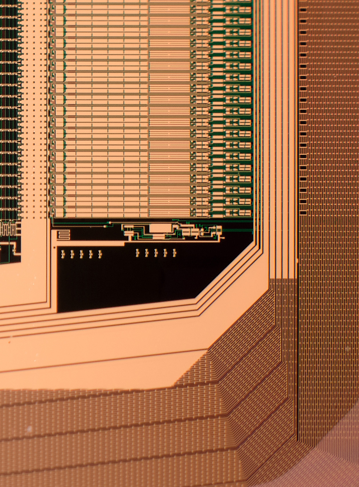

This one should be much easier to guess than last month’s ware; it’s strategically cropped to add a tiny bit of challenge to it. I’ll add some more views of the ware once we’ve got a correct answer.

I was really struck by the quality of the photography of this ware. jackw01 submitted a series of wares (this one included), which I’ll be sharing over the coming months. I have a lot to learn about photography, and I thought it might be of general interest to hear his answer on how this ware was photographed:

[The ware] was shot with a Fujifilm X-T30 using a 40-year-old Canon FD mount 50mm prime lens with a set of 10+16mm macro extension tubes. If you’re unfamiliar, extension tubes are basically a way of achieving macro photography without having a dedicated macro lens. They decrease the minimum focusing distance and increase the magnification of a lens according to the ratio between the length of the extension tube and the focal length of the lens, producing 1:1 magnification when the extension tube length equals the focal length. When using both the 10 and 16mm extension tubes together with the 18-55mm lens, my usable field of view is anywhere from 25-50mm wide depending on the focal length and focus distance with the subject ~0-20mm away from the lens, and with the 50mm prime, the field of view is 30-45mm wide with the subject 70-90mm away from the lens. When using extension tubes, I would highly recommend using manual focus, even though most extension tubes have the electrical connections to support autofocus – the autofocus algorithms on most cameras are just not tuned to work with extension tubes and often won’t focus at all or won’t produce as sharp of an image.

Thanks again to jackw01 for sharing this ware, and for sharing your know-how on photographing them!

Winner, Name that Ware September 2021

Wow! The ware for September 2021 was a real stumper. To be honest, when Marcan showed me the wares, I had similar instincts to most of those who entered guesses — I was entirely thrown off by the spendy choice of components combined with the huge array of multimedia connectors. Before seeing this ware, I never associated “karaoke” with “expensive electronics”; well, maybe this is a datapoint on how lucrative a business karaoke must be.

TL;DR: The Ware is a Joysound F1, and the winner is Thorkell, who finally managed to piece together the puzzle the day before the contest was scheduled to end. Calvin was actually the first to guess the correct genre of the machine, but Thorkell came as close as possible given the provided images to correctly identifying the make and model (not enough info was in the photos to reveal if it was the f1 or the fR model). Congrats, email me for your well-earned prize!

Marcan, who you should definitely follow if you have any interest in Linux, reverse engineering, and/or the M1 from Apple (he will be live-streaming an Asahi Linux bring-up on Nov 1!), also kindly provided this very detailed write-up on the ware:

Marcan’s Insights on the Joysound f1

This is a Joysound f1 (codename “Ken”), one of the more popular karaoke machines used in shops across Japan. It was released in 2012. You’re likely to have used one if you’ve been around more than once or twice. There are, to my knowledge, no previous teardowns of these machines on the internet, so I was intrigued by how they worked. I picked one up in an auction, and I will say I was not expecting what I saw when I tore it apart!

These machines are “networked karaoke” and periodically call home to update the song database (and require an ongoing subscription to work), but they are designed to work on anything from FTTH to periodic dial-up connections, so they need to have all the data locally. To that end, there’s a big 3TB hard disk with (almost) the entire song database (it is subsetted differently depending on your network speed, e.g. you won’t get many background videos on dial-up, and songs published as user submissions are always streamed on-demand and available only on broadband configurations). The HDD also contains firmware, updates, and anything else that needs pushing out to machines. As of the August update they seem to be using 2.5TB of the storage capacity, so it’s pretty tight already!

The architecture is bizarre. The Tegra 2 SoM is the main processor of the system, running Linux4Tegra (Ubuntu 10.10 ARM32) with good old Xorg; it is in charge of the main karaoke playback, networking, updates, remote control service, etc. Interestingly, it can also peer with another machine to serve its data over the network, which is useful when an HDD dies, to avoid having to take the machine out of service entirely. It boots off of a ramdisk loaded off of the HDD, and quite impressively, the entire rootfs is less than 150MB uncompressed. Control is usually via external touchscreen or tablet remotes, that connect typically via an external Wi-Fi access point and network, but can also use the internal Wi-Fi card in ad-hoc mode.

The entire audio subsystem is offloaded to the Roland board, which has a full MIDI synthesizer (for the karaoke; most songs are MIDI, although AAC is also supported and decoded by the Tegra before being pushed to the Roland as PCM) and DSP engine for Mic effects (reverb, voice changer, anti-howling, etc). In fact, it even has a fancy system for using an external microphone to measure the acoustic characteristics of the room and automatically compute a DSP profile. On top of the core MIDI patches, the Tegra also uploads an extra set of very high quality bass and drum samples to the Roland via the USB connection. Talk about high-end MIDI!

All the I/O is for things like the mics, external background music/video sources, instrument inputs (e.g. you can add a guitar preamp frontend), and auxiliary outputs. This is the first machine in its range to have HDMI, so it only has a single output; a newer revision called F1v added an HDMI input and dual HDMI outputs, to allow for HDMI idle/background video feeds.

The front touch panel is driven by the Marvell Armada SoC and is its own system running Android Eclair. It gets an SD feed of the main system’s video to display when idle, and it can composite its menus on top. It is otherwise a completely standalone system, with its own song metadata database updated from the main unit, etc. It communicates with the main system chiefly via USB networking and some of the same APIs that external Wi-Fi remotes would use. This is the first machine from Joysound to have an embedded touchscreen interface, and basically what they did was take the existing JR-300 “Mary” stand-alone touchscreen remote and embed it into the main unit. They call it “pamary” (Panel Mary, presumably). Amusingly, the ad-hoc Wi-Fi dongle is connected to the Armada, not the main SoC, so external remotes connected in this way end up routing through it into the main SoC. No idea why they did it like that.

The next generation (Joysound MAX “Zeus”) is basically an iteration of the same architecture. They ditched the Tegra 2 and replaced it with a Renesas R-Car-H2 (keeping with the automotive SoC theme…) and the distro is now Yocto-based, but the front panel SoC remains separate. The Roland board is much reduced, presumably using newer more integrated technology. The HDD is now 4TB. There is also a newer MAX2 version, which I don’t have, but I don’t expect it to be much different either.

Thanks for playing this Name That Ware! Hope you enjoyed it!

Name that Ware September 2021

The Ware for September 2021 is shown below.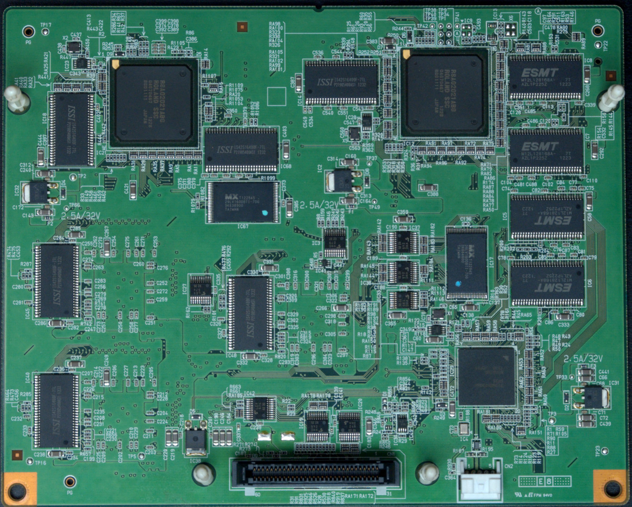

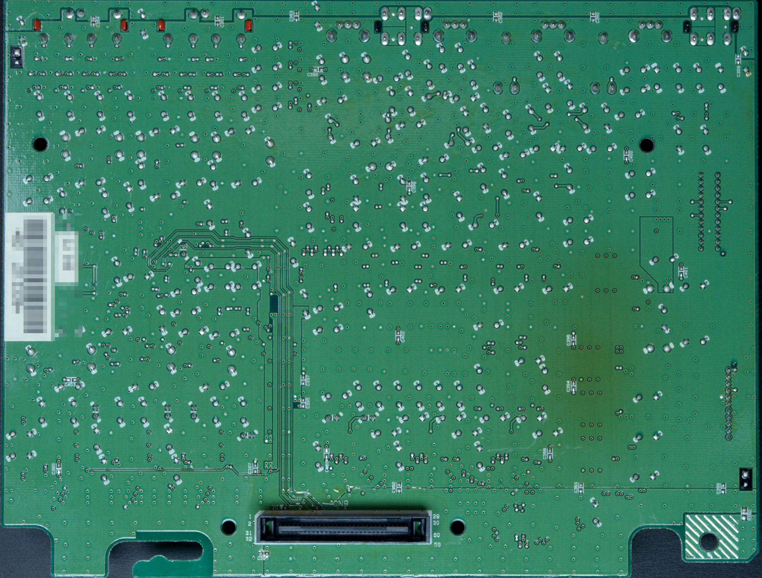
This ware was kindly contributed by @marcan42. I’m really impressed at the quality of the camera work for the wares!

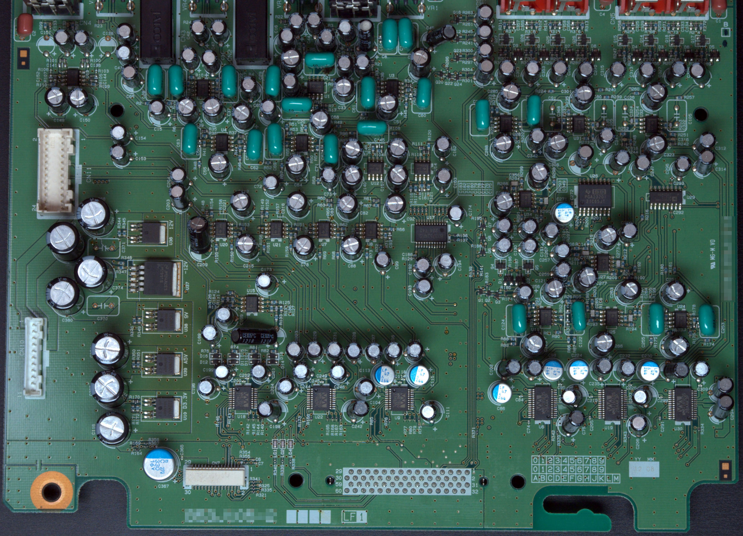
These are just a subset of the boards from the ware, but I suspect it’s more than enough to get a positive ID. The digital board is a bit more telling, but I find a well-designed analog board to be too attractive to pass up posting. I also love the slightly browned regions evidencing the hard life that the linear regulators experienced, filtering out all that power supply junk to create a clean, smooth power rail suitable for audio. If nobody can figure this out, there’s another board I’ll add to the set which might be helpful.

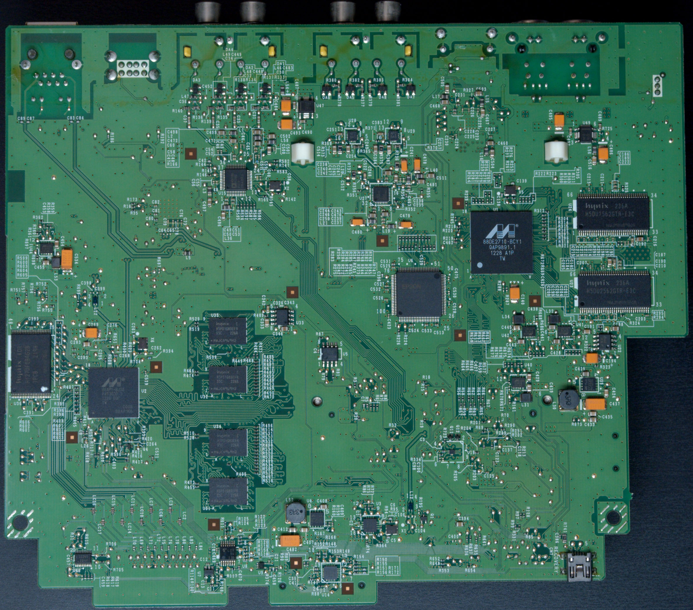
Bonus points to anyone who can come up with a good theory for the ~3mm 45-degree angle cutouts sprinkled around the digital board’s power plane pours. I can’t come up with any consistent rhyme or reason for them to be there, so maybe the engineer was just going for style points? Nothing wrong with going for style, but perhaps I missed the memo on some sort of black magic with respect to detuning resonances in power planes, or something like that.

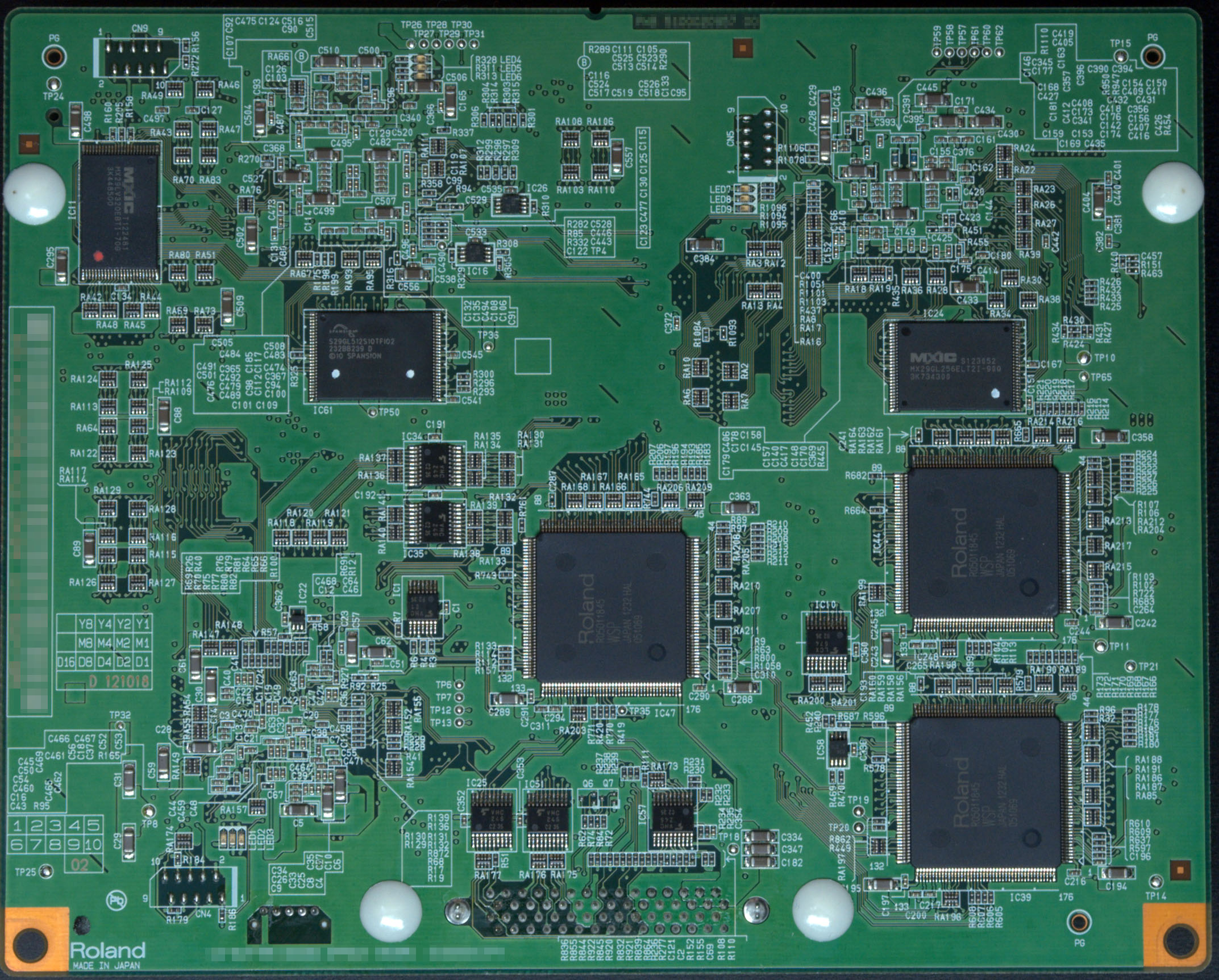
Update Oct 7
It’s been interesting to see where the guesses are going, but unfortunately nobody is getting close. So, here’s another important board from the ware:

Winner, Name that Ware August 2021

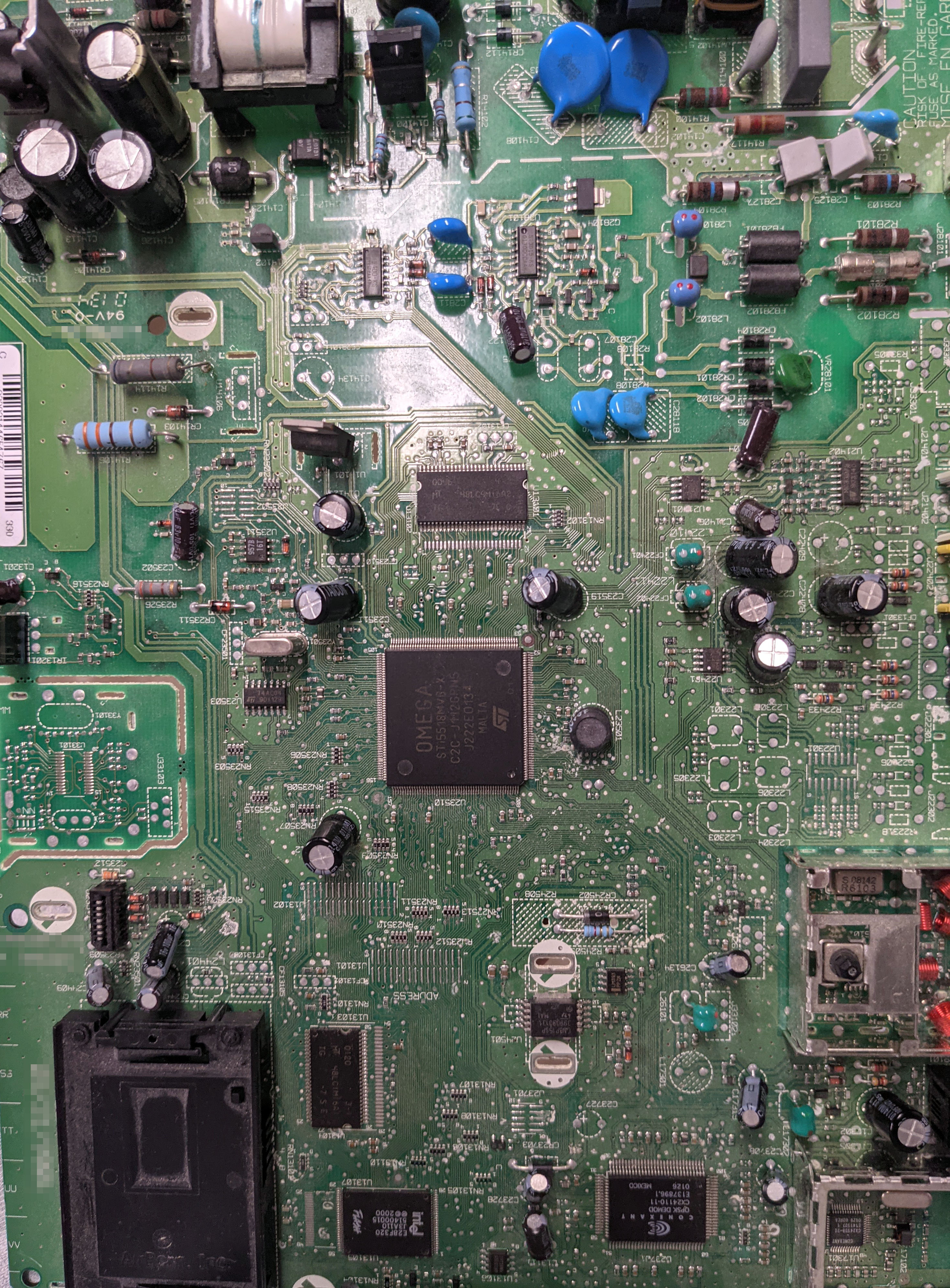
The Ware for August 2021 is a DirectTV receiver model D10. As I had surmised, it was quite easy to guess the nature of the ware, based on obvious clues such as the smart card slot, tuner circuit, and the general TV-receiver-esque vibe about the board. One does not integrate a line voltage power supply and an RF front end into a single circuit board unless one is sure to sell millions of them; the regulatory overhead is just too great otherwise.

Anyways, to make the ware a bit more challenging I had asked for comments specifically about the unpopulated cut-out section of the board. Participants correctly recognized from the get-go that it should be an accessory to the receiver, likely related to a remote control. GotNoTime even went so far as to call out a part number, the KESRX01 ASK receiver chip (as listed in the schematics that were previously linked by Eben Olson). While the schematics share the chip designator U33101, unfortunately, the KESRX01 is a 24-pin package, but the board has a 28-pin footprint. Thus, it’s quite likely these are closely related schematics, probably made by the same OEM, but they also cannot be an exact match.

This motivated me to poke a bit more; a bit of googling around revealed a good match for the footprint and functional category: the TDA5200. Below is a juxtaposition of the reference schematic from the datasheet along with the layout:

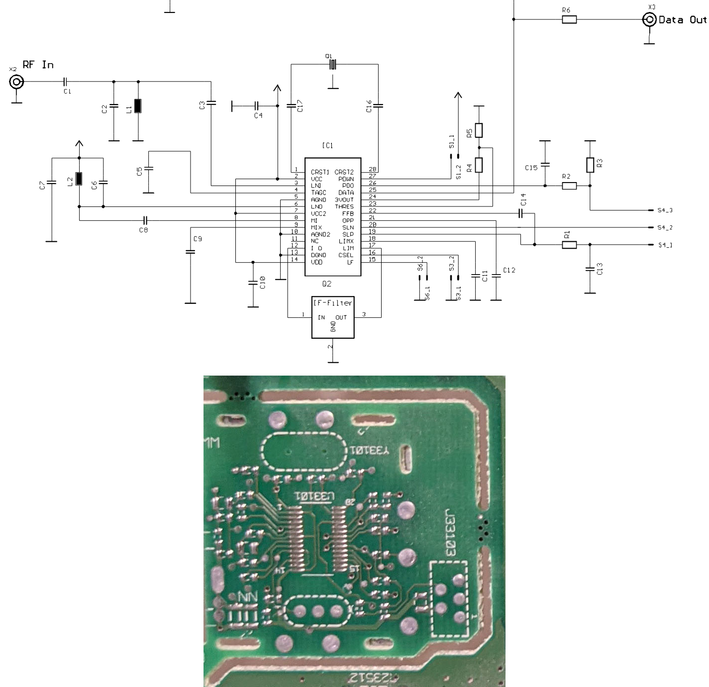
And just for quick reference, here’s the pinout and internal block diagram of the chip: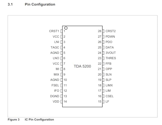

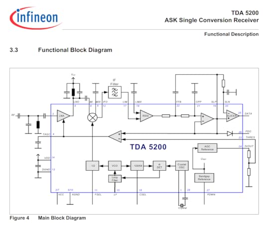
I got as far as confirming that the power supply lines match up, and that the crystal and RF lines seem to make sense, which means it’s likely to be this chip or at least a closely related one. If I had to build up a functional circuit using this board blank and no schematics, I’d say it’s likely to succeed, modulo a couple patch wires and a bit of antenna tuning.

My propensity to figure out what goes into the blank spots of a circuit board is a quirk that stems from having to, at times, reverse engineer devices that have had the part numbers sanded off or obscured for “security” reasons. That’s probably part of the reason I’m drawn toward empty spots on circuit boards; they are good practice for looking at context and circuit traces to figure out part numbers. It’s like circuit board karaoke!

I guess this month there isn’t a winner, since nobody quite got the answer I was looking for, so I’ll leave it at that (although I am probably partially to blame for not being clearer as to what I was hoping to see as an answer!). However, thanks again to everyone for playing!

Name that Ware, August 2021

The Ware for August 2021 is shown below.

This months ware is probably a pretty easy guess. To make things a bit more interesting, the prize will go to the entry that has the most feasible (or the most entertaining!) theory as to the purpose for the tiny break-away, stand-alone PCB is on the left hand side, as indicated by the red arrow. The cropping just barely obscures the edge of the PCB, but basically there are three mouse bites on the edges that retain the sub-assembly PCB, so it could be sheared off and turned into a separate item. I always pay extra attention to blank spots like this PCBs, because they are riddles into some aspect of a product’s design or supply chain: someone put the effort in to design a thing — but then decided not to use it. This PCB has a lot of blank spots, but this is the only one that could be readily sheared off into a separate assembly.

This ware is also a guest ware, courtesy of “JeffA”. Thanks for the submission!

Winner, Name that Ware July 2021

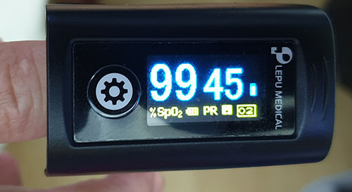
The Ware for July 2021 is a PC-60FW Fingertip Oximeter, which was distributed to each household in Singapore by the Temasek Foundation, free of charge. I thought this was a pretty interesting ware for a few reasons. First, it’s a free oximeter! Kind of a neat thing to play with. You can hold your breath and watch your SPO2 levels go down, or try to meditate and control your pulse.

Second, I found it quite interesting because no where on the box or the manual does it mention that this thing has Bluetooth. Of course, I take apart most things that arrive at my doorstep to see what’s inside — that’s just how I roll. Since it was a free device, I assumed it would probably be a bare-bones implementation, not expecting to see much more than a black glob of epoxy and a few wires when I opened it. Instead, it had these fairly name-brand components, and the antenna came as a bit of a shocker because I didn’t expect any sort of telemetry from the device. The box bears no indication of a radio transmitter — there’s no EMC-compliance notice, MAC address, icons, or any kind of verbiage that would typically compliment a radio transmitter. Must be nice to be able to ship millions of units of a product without having to deal with EMC compliance. After a careful inspection of the manual, however, there is a reference to the fact that you could download the “@Health” app, which includes a QR code to a random website to side-load an APK into your phone from “Shenzhen Creative”.

I’m not quite sure what was the thought behind including the Bluetooth function — it’s not cheap, especially for a nationwide-scale deployment. I would have assumed they were going to integrate this into their “Healthhub” app which is the official government app for managing healthcare, to allow them an opportunity to triage COVID cases before bringing them into the ward. However, I didn’t investigate the @Health app any further; it was served from a Chinese-style domain name I didn’t recognize, without https, etc. etc. I don’t have the time to deal with disassembling the app to make sure it’s clean before installing it, so I just steered clear of it. A Nordic Bluetooth radio on its own isn’t a perilous surveillance threat, due to its limited range and capability. However, once paired with a smartphone app, the scope of the data goes global and the threat is much more severe due to the potential for data fusion with the smartphone’s sensors, and other private data within.

Anyways, I found it a bit surprising that my pulse oximeter has a radio, and thought it’d be a neat ware to share!

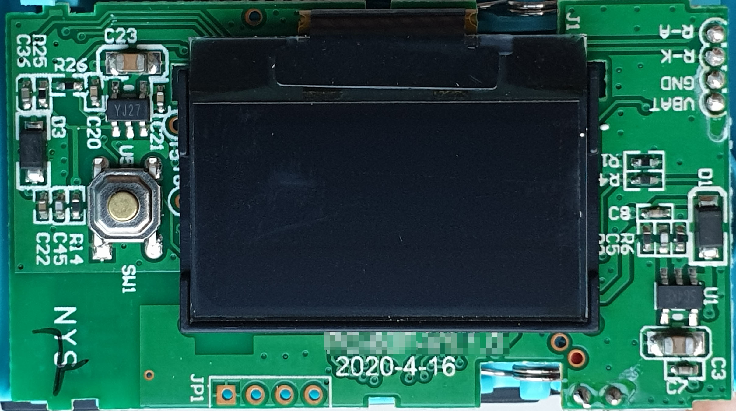
This is a picture of the “less-interesting” side of the oximeter PCB. It uses the same OLED display that found its way into the $12 Shanzhai phones from the turn of the millennium. That characteristic cyan-and-amber color scheme seems to be the “go-to” display for budget-conscious IoT devices these days.

Bienvenu is the clear winner on guessing this one, congrats! email me for your prize.

Name that Ware, July 2021

The Ware for July 2021 is shown below.
[image error]
For well over a year now, I haven’t traveled much further than 10km from where I sit and write this. However, sometimes the world brings you interesting things. This ware has a little bit of a story behind it; it arrived, and of course I popped off the cover to see what was inside. It wasn’t quite what I was expecting to see — more on that, after we’ve given some time for people to share their guesses! I imagine this could be a fairly easy one to guess, as most of the components involved in its core functionality are in this view.

Winner, Name that Ware June 2021

The Ware for June 2021 is an Amplifier Research AR200L 200W linear power amp. This is the last (for now at least) of the very fine set of wares that Don Straney had contributed. Thanks, Don! They helped get me through the pandemic, until I can travel the world again and stumble across new wares. Unfortunately, the delta variant means any hope of travel in the near term is probably off the table. But! I still have a screw driver, so I’ll be scouring my place for interesting things to photograph and share.

I’ll pick Phantom Deadline as the winner for last month’s competition, congrats and email me for your prize! I found the comment thread to be very interesting to read; I’m a decade too young to have learned how to design with vacuum tubes in college, and I never picked up tube design later on. For me, at least, I had no idea what I was staring at when I saw the ware initially. So, I appreciated the discussion of vacuum tube RF design tricks. Thanks to everyone who commented, for teaching me new things!

Building a Curve25519 Hardware Accelerator

Note: this post uses a $\LaTeX$ plugin to render math symbols. It may require a desktop browser for the full experience…

The “double ratchet” algorithm is integral to modern end-to-end-encrypted chat apps, such as Signal, WhatsApp, and Matrix. It gives encrypted conversations the properties of resilience, forward secrecy, and break-in recovery; basically, even if an adversary can manipulate or observe portions of an exchange, including certain secret materials, the damage is limited with each turn of the double ratchet.

The double-ratchet algorithm is a soup of cryptographic components, but one of the most computationally expensive portions is the “Diffie-Hellman (DH) key exchange”, using Elliptic Curve Diffie-Hellman (ECDH) with Curve25519. How expensive? This post from 2020 claims a speed record of 3.2 million cycles on a Cortex-M0 for just one of the core mathematical operations: fairly hefty. A benchmark of the x25519-dalek Rust crate on a 100 MHz RV32-IMAC implementation clocks in at 100ms per DH key exchange, of which several are involved in a double-ratchet. Thus, any chat client implementation on a small embedded CPU would suffer from significant UI lag.

There are a few strategies to rectify this, ranging from adding a second CPU core to off-load the crypto, to making a full-custom hardware accelerator. Adding a second RISC-V CPU core is expedient, but it wouldn’t do much to force me to understand what I was doing as far as the crypto goes; and there’s already a strong contingent of folks working on multi-core RISC-V on FPGA implementations. The last time I implemented a crypto algorithm was for RSA on a low-end STM32 back in the mid 2000’s. I really enjoyed getting into the guts of the algorithm and stretching my understanding of the underlying mathematical primitives. So, I decided to indulge my urge to tinker, and make a custom hardware accelerator for Curve25519 using Litex/Migen and Rust bindings.

What the Heck Is $\mathbf{{F}}_{{{{2^{{255}}}}-19}}$?

I wanted the accelerator primitive to plug directly into the Rust Dalek Cryptography crates, so that I would be as light-fingered as possible with respect to changes that could lead to fatal flaws in the broader cryptosystem. I built some simple benchmarks and profiled where the most time was being spent doing a double-ratchet using the Dalek Crypto crates, and the vast majority of the time for a DH key exchange was burned in the Montgomery Multiply operation. I won’t pretend to understand all the fancy math-terms, but people smarter than me call it a “scalar multiply”, and it actually consists of thousands of “regular” multiplies on 255-bit numbers, with modular reductions in the prime field $\mathbf{{F}}_{{{{2^{{255}}}}-19}}$, among other things.

Wait, what? So many articles and journals I read on the topic just talk about prime fields, modular reduction and blah blah blah like it’s asking someone to buy milk and eggs at the grocery store. It was a real struggle to try and make sense of all the tricks used to do a modular multiply, much less to say even elliptic curve point transformations.

Well, that’s the point of trying to implement it myself — by building an engine, maybe you won’t understand all the hydrodynamic nuances around fuel injection, but you’ll at least gain an appreciation for what a fuel injector is. Likewise, I can’t say I deeply understand the number theory, but from what I can tell multiplication in $\mathbf{{F}}_{{{{2^{{255}}}}-19}}$ is basically the same as a “regular 255-bit multiply” except you do a modulo (you know, the `%` operator) against the number $2^{{255}}-19$ when you’re done. There’s a dense paper by Daniel J. Bernstein, the inventor of Curve25519, which I tried to read several times. One fact I gleaned is part of the brilliance of Curve25519 is that arithmetic modulo $2^{{255}}-19$ is quite close to regular binary arithmetic except you just need to special-case 19 outcomes out of $2^{{255}}$. Also, I learned that the prime modulus, $2^{{255}}-19$, is where the “25519” comes from in the name of the algorithm (I know, I know, I’m slow!).

After a whole lot more research I stumbled on a paper by Furkan Turan and Ingrid Verbauwhede that broke down the algorithm into terms I could better understand. Attempts to reach out to them to get a copy of the source code was, of course, fruitless. It’s a weird thing about academics — they like to write papers and “share ideas”, but it’s very hard to get source code from them. I guess that’s yet another reason why I never made it in academia — I hate writing papers, but I like sharing source code. Anyways, the key insight from their paper is that you can break a 255-bit multiply down into operations on smaller, 17-bit units called “limbs” — get it? digits are your fingers, limbs (like your arms) hold multiple digits. These 17-bit limbs map neatly into 15 Xilinx 7-Series DSP48E block (which has a fast 27×18-bit multiplier): 17 * 15 = 255. Using this trick we can decompose multiplication in $\mathbf{{F}}_{{{{2^{{255}}}}-19}}$ into the following steps:

Schoolbook multiplication with 17-bit “limbs”Collapse partial sumsPropagate carriesIs the sum $\geq$ $2^{{255}}-19$?If yes, add 19; else add 0Propagate carries again, in case the addition by 19 causes overflows

The multiplier would run about 30% faster if step (6) were skipped. This step happens in a fairly small minority of cases, maybe a fraction of 1%, and the worst-case carry propagate through every 17-bit limb is diminishingly rare. The test for whether or not to propagate carries is fairly straightforward. However, short-circuiting the carry propagate step based upon the properties of the data creates a timing side-channel. Therefore, we prefer a slower but safer implementation, even if we are spending a bunch of cycles propagating zeros most of the time.

Buckle up, because I’m about to go through each step in the algorithm in a lot of detail. One motivation of the exercise was to try to understand the math a bit better, after all!

TL;DR: Magic Numbers

If you’re skimming this article, you’ll see the numbers “19” and “17” come up over and over again. Here’s a quick TL;DR:

19 is the tiny amount subtracted from $2^{{255}}$ to arrive at a prime number which is the largest number allowed in Curve25519. Overflowing this number causes things to wrap back to 0. Powers of 2 map efficiently onto binary hardware, and thus this representation is quite nice for hardware people like me.17 is a number of bits that conveniently divides 255, and fits into a single DSP hardware primitive (DSP48E) that is available on the target device (Xilinx 7-series FPGA) that we’re using in this post. Thus the name of the game is to split up this 255-bit number into 17-bit chunks (called “limbs”).Schoolbook Multiplication

The first step in the algorithm is called “schoolbook multiplication”. It’s like the kind of multiplication you learned in elementary or primary school, where you write out the digits in two lines, multiply each digit in the top line by successive digits in the bottom line to create successively shifted partial sums that are then added to create the final result. Of course, there is a twist. Below is what actual schoolbook multiplication would be like, if you had a pair of numbers that were split into three “limbs”, denoted as A[2:0] and B[2:0]. Recall that a limb is not necessarily a single bit; in our case a limb is 17 bits.

| A2 A1 A0 x | B2 B1 B0 ------------------------------------------ | A2*B0 A1*B0 A0*B0 A2*B1 | A1*B1 A0*B1 A2*B2 A1*B2 | A0*B2 (overflow) (not overflowing)

The result of schoolbook multiplication is a result that potentially has 2x the number of limbs than the either multiplicand.

Mapping the overflow back into the prime field (e.g. wrapping the overflow around) is a process called reduction. It turns out that for a prime field like $\mathbf{{F}}_{{{{2^{{255}}}}-19}}$, reduction works out to taking the limbs that extend beyond the base number of limbs in the field, shifting them right by the number of limbs, multiplying it by 19, and adding it back in; and if the result isn’t a member of the field, add 19 one last time, and take the result as just the bottom 255 bits (ignore any carry overflow). If this seems magical to you, you’re not alone. I had to draw it out before I could understand it.

This trick works because the form of the field is $2^{{n}}-p$: it is a power of 2, reduced by some small amount $p$. By starting from a power of 2, most of the binary numbers representable in an n-bit word are valid members of the field. The only ones that are not valid field members are the numbers that are equal to $2^{{n}}-p$ but less than $2^{{n}}-1$ (the biggest number that fits in n bits). To turn these invalid binary numbers into members of the field, you just need to add $p$, and the reduction is complete.

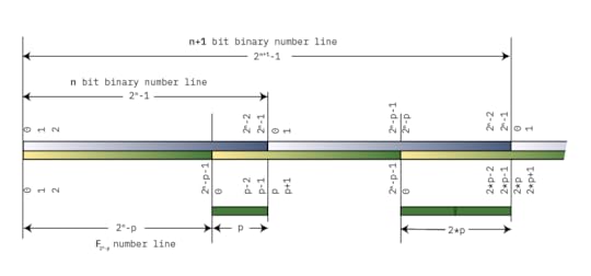
A diagram illustrating modular reduction

The diagram above draws out the number lines for both a simple binary number line, and for some field $\mathbf{{F}}_{{{{2^{{n}}}}-p}}$. Both lines start at 0 on the left, and increment until they roll over. The point at which $\mathbf{{F}}_{{{{2^{{n}}}}-p}}$ rolls over is a distance $p$ from the end of the binary number line: thus, we can observe that $2^{{n}}-1$ reduces to $p-1$. Adding 1 results in $2^{{n}}$, which reduces to $p$: that is, the top bit, wrapped around, and multiplied by $p$.

As we continue toward the right, the numbers continue to go up and wrap around, and for each wrap the distance between the “plain old binary” wrap point and the $\mathbf{{F}}_{{{{2^{{n}}}}-p}}$ wrap point increases by a factor of $p$, such that $2^{{n 1}}$ reduces to $2*p$. Thus modular reduction of natural binary numbers that are larger than our field $2^{{n}}-p$ consists of taking the bits that overflow an $n$-bit representation, shifting them to the right by $n$, and multiplying by $p$.

In order to convince myself this is true, I tried out a more computationally tractable example than $\mathbf{{F}}_{{{{2^{{255}}}}-19}}$: the prime field $\mathbf{{F}}_{{{{2^{{6}}}}-5}} = 59$. The members of the field are from 0-58, and reduction is done by taking any number modulo 59. Thus, the number 59 reduces to 0; 60 reduces to 1; 61 reduces to 2, and so forth, until we get to 64, which reduces to 5 — the value of the overflowed bits (1) times $p$.

Let’s look at some more examples. First, recall that the biggest member of the field, 58, in binary is 0b00_11_1010.

Let’s consider a simple case where we are presented a partial sum that overflows the field by one bit, say, the number 0b01_11_0000, which is decimal 112. In this case, we take the overflowed bit, shift it to the right, multiply by 5:

0b01_11_0000 ^ move this bit to the right multiply by 0b101 (5)0b00_11_0000 0b101 = 0b00_11_0101 = 53

And we can confirm using a calculator that 112 % 59 = 53. Now let’s overflow by yet another bit, say, the number 0b11_11_0000. Let’s try the math again:

0b11_11_0000 ^ move to the right and multiply by 0b101: 0b101 * 0b11 = 0b11110b00_11_0000 0b1111 = 0b00_11_1111

This result is still not a member of the field, as the maximum value is 0b0011_1010. In this case, we need to add the number 5 once again to resolve this “special-case” overflow where we have a binary number that fits in $n$ bits but is in that sliver between $2^{{n}}-p$ and $2^{{n}}-1$:

0b00_11_1111 0b101 = 0b01_00_0100

At this step, we can discard the MSB overflow, and the result is 0b0100 = 4; and we can check with a calculator that 240 % 59 = 4.

Therefore, when doing schoolbook multiplication, the partial products that start to overflow to the left can be brought back around to the right hand side, after multiplying by $p$, in this case, the number 19. This magical property is one of the reasons why $\mathbf{{F}}_{{{{2^{{255}}}}-19}}$ is quite amenable to math on binary machines.

Let’s use this finding to rewrite the straight schoolbook multiplication form from above, but now with the modular reduction applied to the partial sums, so it all wraps around into this compact form:

| A2 A1 A0 x | B2 B1 B0 ------------------------------------------ | A2*B0 A1*B0 A0*B0 | A1*B1 A0*B1 19*A2*B1 | A0*B2 19*A2*B2 19*A1*B2 ---------------------------- S2 S1 S0

As discussed above, each overflowed limb is wrapped around and multiplied by 19, creating a number of partial sums S[2:0] that now has as many terms as there are limbs, but with each partial sum still potentially overflowing the native width of the limb. Thus, the inputs to a limb are 17 bits wide, but we retain precision up to 48 bits during the partial sum stage, and then do a subsequent condensation of partial sums to reduce things back down to 17 bits again. The condensation is done in the next three steps, “collapse partial sums”, “propagate carries”, and finally “normalize”.

However, before moving on to those sections, there is an additional trick we need to apply for an efficient implementation of this multiplication step in hardware.

In order to minimize the amount of data movement, we observe that for each row, the “B” values are shared between all the multipliers, and the “A” values are constant along the diagonals. Thus we can avoid re-loading the “A” values every cycle by shifting the partial sums diagonally through the computation, allowing the “A” values to be loaded as “A” and “A*19” into holding register once before the computations starts, and selecting between the two options based on the step number during the computation.

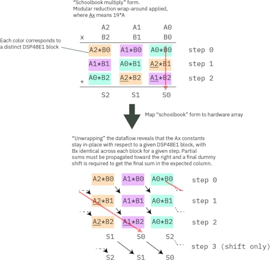
Mapping schoolbook multiply onto the hardware array to minimize data movement

The diagram above illustrates how the schoolbook multiply is mapped onto the hardware array. The top diagram is an exact redrawing of the previous text box, where the partial sums that would extend to the left have been multiplied by 19 and wrapped around. Each colored block corresponds to a given DSP48E1 block, which you may recall is a fast 27×18 multiplier hardware primitive built into our Xilinx FPGAs. The red arrow illustrates the path of a partial sum in both the schoolbook form and the unwrapped form for hardware implementation. In the bottom diagram, one can clearly see that the Ax coefficients are constant for each column, and that for each row, the Bx values are identical across all blocks in each step. Thus each column corresponds to a single DSP48E1 block. We take advantage of the ability of the DSP48E1 block to hold two selectable A values to pre-load Ax and Ax*19 before the computation starts, and we bus together the Bx values and change them in sequence with each round. The partial sums are then routed to the “down and right” to complete the mapping. The final result is one cycle shifted from the canonical mapping.

We have a one-cycle structural pipeline delay going from this step to the next one, so we use this pipeline delay to do a shift with no add by setting the `opmode` from `C M` to `C 0` (in other words, instead of adding to the current multiplication output for the last step, we squash that input and set it to 0).

The fact that we pipeline the data also gives us an opportunity to pick up the upper limb of the partial sum collapse “for free” by copying it into the “D” register of the DSP48E1 during the shift step.

In C, the equivalent code basically looks like this:

// initialize the a_bar set of data for( int i = 0; i < DSP17_ARRAY_LEN; i ) {{ a_bar_dsp[i] = a_dsp[i] * 19; }} operand p; for( int i = 0; i < DSP17_ARRAY_LEN; i ) {{ p[i] = 0; }} // core multiply for( int col = 0; col < 15; col ) {{ for( int row = 0; row < 15; row ) {{ if( row >= col ) {{ p[row] = a_dsp[row-col] * b_dsp[col]; }} else {{ p[row] = a_bar_dsp[15 row-col] * b_dsp[col]; }} }} }}

By leveraging the special features of the DSP48E1 blocks, in hardware this loop completes in just 15 clock cycles.

Collapse Partial Sums

At this point, the potential width of the partial sum is up to 43 bits wide. This next step divides the partial sums up into 17-bit words, and then shifts the higher to the next limbs over, allowing them to collapse into a smaller sum that overflows less.

... P2[16:0] P1[16:0] P0[16:0]... P1[33:17] P0[33:17] P14[33:17]*19... P0[50:34] P14[50:34]*19 P13[50:34]*19

Again, the magic number 19 shows up to allow sums which “wrapped around” to add back in. Note that in the timing diagram you will find below, we refer to the mid- and upper- words of the shifted partial sums as “Q” and “R” respectively, because the timing diagram lacks the width within a data bubble to write out the full notation: so `Q0,1` is P14[33:17] and `R0,2` is P13[50:34] for P0[16:0].

Here’s the C code equivalent for this operation:

// the lowest limb has to handle two upper limbs wrapping around (Q/R) prop[0] = (p[0] & 0x1ffff) (((p[14] * 1) >> 17) & 0x1ffff) * 19 (((p[13] * 1) >> 34) & 0x1ffff) * 19; // the second lowest limb has to handle just one limb wrapping around (Q) prop[1] = (p[1] & 0x1ffff) ((p[0] >> 17) & 0x1ffff) (((p[14] * 1) >> 34) & 0x1ffff) * 19; // the rest are just shift-and-add without the modular wrap-around for(int bitslice = 2; bitslice < 15; bitslice = 1) {{ prop[bitslice] = (p[bitslice] & 0x1ffff) ((p[bitslice - 1] >> 17) & 0x1ffff) ((p[bitslice - 2] >> 34)); }}

This completes in 2 cycles after a one-cycle pipeline stall delay penalty to retrieve the partial sum result from the previous step.

Propagate Carries

The partial sums will generate carries, which need to be propagated down the chain. The C-code equivalent of this looks as follows:

for(int i = 0; i < 15; i ) {{ if ( i 1 < 15 ) {{ prop[i 1] = (prop[i] >> 17) prop[i 1]; prop[i] = prop[i] & 0x1ffff; }} }}

The carry-propagate completes in 14 cycles. Carry-propagates are expensive!

Normalize

We’re almost there! Except that $0 \leq result \leq 2^{{256}}-1$, which is slightly larger than the range of $\mathbf{{F}}_{{{{2^{{255}}}}-19}}$.

Thus we need to check if number is somewhere in between 0x7ff….ffed and 0x7ff….ffff, or if the 256th bit will be set. In these cases, we need to add 19 to the result, so that the result is a member of the field $2^{{255}}-19$ (the 256th bit is dropped automatically when concatenating the fifteen 17-bit limbs together into the final 255-bit result).

We use another special feature of the DSP48E1 block to help accelerate the test for this case, so that it can complete in a single cycle without slowing down the machine. We use the “pattern detect” (PD) feature of the DSP48E1 to check for all “1’s” in bit positions 255-5, and a single LUT to compare the final 5 bits to check for numbers between {prime_string} and $2^{{255}}-1$. We then OR this result with the 256th bit.

If the result falls within this special “overflow” case, we add the number 19, otherwise, we add 0. Note that this add-by-19-or-0 step is implemented by pre-loading the number 19 into the A:B pipeline registers of the DSP4E1 block during the “propagate” stage. Selection of whether to add 19 or 0 relies on the fact that the DSP48E1 block has an input multiplexer to its internal adder that can pick data from multiple sources, including the ability to pick no source by loading the number 0. Thus the operation mode of the DSP48E1 is adjusted to either pull an input from A:B (that is, the number 19) or the number 0, based on the result of the overflow computation. Thus the PD feature is important in preventing this step from being rate-limiting. With the PD feature we only have to check an effective 16 intermediate results, instead of 256 raw bits, and then drive set the operation mode of the ALU.

With the help of the special DSP48E1 features, this operation completes in just a single cycle.

After adding the number 19, we have to once again propagate carries. Even if we add the number 0, we also have to “propagate carries” for constant-time operation, to avoid leaking information in the form of a timing side-channel. This is done by running the carry propagate operation described above a second time.

Once the second carry propagate is finished, we have the final result.

Potential corner case

There is a potential corner case where if the carry-propagated result going into “normalize” is between

0xFFFF_FFFF_FFFF_FFFF_FFFF_FFFF_FFFF_FFDA and0xFFFF_FFFF_FFFF_FFFF_FFFF_FFFF_FFFF_FFEC

In this case, the top bit would be wrapped around, multiplied by 19, and added to the LSB, but the result would not be a member of $2^{{255}}-19$ (it would be one of the 19 numbers just short of $2^{{255}}-1$), and the multiplier would pass it on as if it were a valid result.

In some cases, this isn’t even a problem, because if the subsequent result goes through any operation that also includes a reduce operation, the result will still reduce correctly.

However, I do not think this corner case is possible, because the overflow path to set the high bit is from the top limb going from 0x1_FFFF -> 0x2_0000 (that is, 0x7FFFC -> 0x80000 when written MSB-aligned) due to a carry coming in from the lower limb, and it would require the carry to be very large, not just 1 as shown in the simple rollover case, but a value from 0x1_FFED-0x1_FFDB.

I don’t have a formal mathematical proof of this, but I strongly suspect that carry values going into the top limb cannot approach these large numbers, and therefore it is not possible to hit this corner case. Consider that the biggest value of a partial sum is 0x53_FFAC_0015 (0x1_FFFF * 0x1_FFFF * 15). This means the biggest value of the third overflowed 17-bit limb is 0x14. Therefore the biggest value resulting from the “collapse partial sums” stage is 0x1_FFFF 0x1_FFFF 0x14 = 0x4_0012. Thus the largest carry term that has to propagate is 0x4_0012 >> 17 = 2. 2 is much smaller than the amount required to trigger this condition, that is, a value in the range of 0x1_FFED-0x1_FFDB. Thus, perhaps this condition simply can’t happen? It’d be great to have a real mathematician comment if this is a real corner case…

Real Hardware

You can jump to the actual code that implements the above algorithm, but I prefer to think about implementations visually. Thus, I created this timing diagram that fully encapsulates all of the above steps, and the data movements between each part (click on the image for an editable, larger version; works best on desktop):

> 17 ","C* >> 17 "]}, { "name": "dsp.d", "wave": "x.........55x.xxxxxx...xxxxxxx.", "data":["*Q0,1","R0,2"]}, {}, { "name": "A1_CE", "wave": "1.010.....10..................." }, { "name": "A1", "wave": "x.2.2......8.........x.........", "data": ["A0xx","A0xx*19","0"] }, { "name": "A2_CE", "wave": "0..10......10.................." }, { "name": "A2", "wave": "x...2.......8........x.........", "data":["A0xx","0"] }, { "name": "B2_CE", "wave": "01.......01.0......10.........." }, { "name": "B2", "wave": "x.22===|==x55xxxx.xx8x.........", "data": ["19","B00","B01","B02","B03","B13","B14","1or19","1or19","19"] }, { "name": "C", "wave": "x...2===|==555...|..86...|..x..", "data": ["Q0","Q1","Q2","Q3","Q13","Q14","P0,0","*P","C* >> 17 ","C&","C* >> 17 "] }, { "name": "D_CE", "wave": "0.........1.0.................." }, { "name": "D", "wave": "x..........55xx................", "data": ["Q0,1","R0,2","QS14,1","RS14,2","QS14,1","RS14,2"] }, { "name": "inmode", "wave": "x.2.2.....x5.x.xx.xx8x.........", "data":["A1B2","AnB2","DB2","0B2"]}, { "name": "opmode", "wave": "x.2.=.....2555...|..86...|..xxx", "data":["M","C+M","C+0","C+M","P+M","C+P","AB/0+C","C+P"]}, {}, { "name": "P_CE", "wave": "0.1.....|....5555|5516666|660.1", "data": ["P1", "P2", "P3","P4","P13","P14","P1", "P2", "P3","P4","P13","P14"] }, { "name": "P", "wave": "x..2====|===55555|5552666|666x.", "data": ["A19","P0","P1","P2","P3","P13","P14","P0","PLSB","PMSB","C1","C2","C3","C12", "C13","C14","S+","C1","C2","C3","C12", "C13","C14","final"] }, { "name": "overflow", "wave": "x...................2x.........", "data":["Y/N"]}, { "name": "done", "wave": "0...........................10." }, ]}">[image error]

Block diagrams of the multiplier and even more detailed descriptions of its function can be found in our datasheet documentation. There’s actually a lot to talk about there, but the discussion rapidly veers into trade-offs on timing closure and coding technique, and farther away from the core topic of the Curve25519 algorithm itself.

Didn’t You Say We Needed Thousands of These…?

So, that was the modular multiply. We’re done right? Nope! This is just one core op in a sequence of thousands of these to do a scalar multiply. One potentially valid strategy could be to try to hang the modular multiplier off of a Wishbone bus peripheral and shove numbers at it, and come back and retrieve results some time later. However, the cost of pushing 256-bit numbers around is pretty high, and any gains from accelerating the multiply will quickly be lost in the overhead of marshaling data. After all, a recurring theme in modern computer architecture is that data movement is more expensive than the computation itself. Damn you, speed of light!

Thus, in order to achieve the performance I was hoping to get, I decided to wrap this inside a microcoded “CPU” of sorts. Really more of an “engine” than a car — if a RISC-V CPU is your every-day four-door sedan optimized for versatility and efficiency, the microcoded Curve25519 engine I created is more of a drag racer: a turbocharged engine block on wheels that’s designed to drive long flat stretches of road as fast as possible. While you could use this to drive your kids to school, you’ll have a hard time turning corners, and you’ll need to restart the engine after every red light.

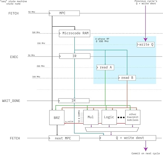
Above is a block diagram of the engine’s microcoded architecture. It’s a simple “three-stage” pipeline (FETCH/EXEC/RETIRE) that runs at 50MHz with no bypassing (that would be extremely expensive with 256-bit wide datapaths). I was originally hoping we could close timing at 100MHz, but our power-optimized -1L FPGA just wouldn’t have it; so the code sequencer runs at 50MHz; the core multiplier at 100MHz; and the register file uses four phases at 200MHz to access a simple RAM block to create a space-efficient virtual register file that runs at 50MHz.

The engine has just 13 opcodes:

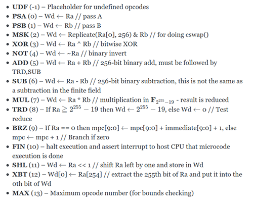
There’s no compiler for it; instead, we adapted the most complicated Rust macro I’ve ever seen from johnas-schievink’s rustasm6502 crate to create the abomination that is engine25519-as. Here’s a snippet of what the assembly code looks like, in-lined as a Rust macro:

let mcode = assemble_engine25519!(start: // from FieldElement.invert() // let (t19, t3) = self.pow22501(); // t19: 249..0 ; t3: 3,1,0 // let t0 = self.square(); // 1 e_0 = 2^1 mul %0, 0, 0 // self is W, e.g. 0 // let t1 = t0.square().square(); // 3 e_1 = 2^3 mul %1, %0, %0 mul %1, %1, %1 // let t2 = self * &t1; // 3,0 e_2 = 2^3 2^0 mul %2, 0, %1 // let t3 = &t0 * &t2; // 3,1,0 mul %3, %0, %2 // let t4 = t3.square(); // 4,2,1 mul %4, %3, %3 // let t5 = &t2 * &t4; // 4,3,2,1,0 mul %5, %2, %4 // let t6 = t5.pow2k(5); // 9,8,7,6,5 psa (, #5 // coincidentally, constant #5 is the number 5 mul %6, %5, %5pow2k_5: sub (, (, #1 // ( = ( - 1 brz pow2k_5_exit, ( mul %6, %6, %6 brz pow2k_5, #0pow2k_5_exit: // let t7 = &t6 * &t5; // 9,8,7,6,5,4,3,2,1,0 mul %7, %6, %5);

The `mcode` variable is a [i32] fixed-length array, which is quite friendly to our `no_std` Rust environment that is Xous.

Fortunately, the coders of the curve25519-dalek crate did an amazing job, and the comments that surround their Rust code map directly onto our macro language, register numbers and all. So translating the entire scalar multiply inside the Montgomery structure was a fairly straightforward process, including the final affine transform.

How Well Does It Run?

The fully accelerated Montgomery multiply operation was integrated into a fork of the curve25519-dalek crate, and wrapped into some benchmarking primitives inside Xous, a small embedded operating system written by Xobs. A software-only implementation of curve25519 would take about 100ms per DH operation on a 100MHz RV32-IMAC CPU, while our hardware-accelerated version completes in about 6.7ms — about a 15x speedup. Significantly, the software-only operation does not incur the context-switch to the sandboxed hardware driver, whereas our benchmark includes the overhead of the syscall to set up and run the code; thus the actual engine itself runs a bit faster per-op than the benchmark might hint at. However, what I’m most interested in is in-application performance, and therefore I always include the overhead of swapping to the hardware driver context to give an apples-to-apples comparison of end-user application performance. More importantly, the CPU is free to do other things while the engine does it’s thing, such as servicing the network stack or updating the UX.

I think the curve25519 accelerator engine hit its goals — it strapped enough of a rocket on our little turtle of a CPU so that it’ll be able render a chat UX while doing double-ratchets as a background task. I also definitely learned more about the algorithm, although admittedly I still have a lot more to learn if I’m to say I truly understand elliptic curve cryptography. So far I’ve just shaken hands with the fuzzy monsters hiding inside the curve25519 closet; they seem like decent chaps — they’re not so scary, I just understand them poorly. A couple more interactions like this and we might even become friends. However, if I were to be honest, it probably wouldn’t be worth it to port the curve25519 accelerator engine from its current FPGA format to an ASIC form. Mask-defined silicon would run at least 5x faster, and if we needed the compute power, we’d probably find more overall system-level benefit from a second CPU core than a domain-specific accelerator (and hopefully by then the multi-core stuff in Litex will have sufficiently stabilized that it’d be a relatively low-risk proposition to throw a second CPU into a chip tape-out).

That being said, I learned a lot, and I hope that by sharing my experience, someone else will find Curve25519 a little more approachable, too!