Paul Gilster's Blog, page 38

Energetics of Archaean Life in the Ocean Vents

If SETI is all about intelligence, and specifically technology, at the other end of astrobiology is the question of abiogenesis. Does life of any kind in fact occur elsewhere, or does Earth occupy a unique space in the scheme of things? Alex Tolley looks today at one venue where life may evolve, deep inside planetary crusts, with implications that include what we may find “locally” at places like Europa or Titan. In doing so, he takes a deep dive into a new paper from Jeffrey Dick and Everett Shock, while going on to speculate on broader questions forced by life’s emergence. Organisms appearing in the kind of regions we are discussing today would doubtless be undetectable by our telescopes, but with favorable energetics, deep ocean floors may spawn abundant life outside the conventional habitable zone, just as they have done within our own ‘goldilocks’ world.

by Alex Tolley

Are the deep hot ocean vents more suitable for life than previously thought?

In a previous article [1] I explored the possibility that while we think of hot planetary cores, and tidal heating of icy moons, as the driver to maintain liquid water and potentially support chemotrophic life at the crust-ocean interface, radiolysis can also provide the means to do the same and allow life to exist at depth in the crust despite the most hostile of surface conditions. On Earth we have the evidence that there is a lithospheric biosphere that extends to a depth of over 1 kilometer, and the geothermal gradient suggests that extremophiles could live several kilometers down in the crust.

Scientists are actively searching for biosignatures in the crust of Mars, away from the UV, radiation, and toxic conditions on the surface examined by previous landers and rovers. Plans are also being drawn up to look for biosignatures in Jupiter’s icy moon Europa, where hot vents at the bottom of a subsurface ocean could host life. It is hypothesized that Titan may have liquid water at depth below its hydrocarbon surface, and even frozen Pluto may have liquid water deep below its surface of frozen gases. The dwarf planet Ceres also may have a slushy, salty ocean beneath its surface as salts left by cryovolcanism indicate. Conditions conducive to supporting life may be common once we look beyond the surface conditions, and therefore subsurface biospheres might be more common than our terrestrial one.

Image: Rainbow vent field. Credit: Royal Netherlands Institute for Sea Research.

The conditions of heat and ionizing radiation at depth, coupled with the appropriate geology, and water, are energetically favorable to split hydrogen (H2) from water, and then reduce carbon dioxide (CO2) to methane (CH4) via the serpentinization reaction. Chemotrophs feed on this reduced carbon as fuel to power their metabolisms. This reaction has an energy barrier that results in more reactants than products than would be expected at equilibrium. As the reaction energetics are favorable, life also evolves to exploit those reactions, with catalytic metabolic pathways that overcome the energy barrier and allow the equilibrium to be reached, realising the reaction energy..

Biologists now classify life into 3 domains: bacteria, eukaryotes, and the archaea. The bacteria are an extremely diverse group that represent the most species on Earth. They can transfer genes between species, allowing for rapid evolution and adaptation to conditions. [It is this horizontal gene transfer that can create antibiotic resistance in bacteria never previously exposed to these treatments.] The eukaryotes, which include the plants, animals and fungi, range from the single cell organisms such as yeast and photosynthetic cyanobacteria, to complex organisms including all the main animal phyla from spongers to vertebrates. The archaea were only relatively recently (1977) recognized as a distinct domain, separate from the bacteria. Archaea include many of the extremophiles, but perhaps most importantly, exploit the reduction of CO2 with H2 to produce CH4. These archaea are called autotrophic methanogens and require anaerobic conditions. The CH4 is released into the environment, just as plants release oxygen (O2) from photosynthesis. In close proximity to the hot, reducing ocean vent conditions, cold, oxygenated seawater supports aerobic metabolisms, resulting in a biologically rich ecosystem, despite the almost lightless conditions in the abyssal ocean depths.

While CH4 and other reduced carbon compounds are both abiotically and biotically produced, we tend to assume that the formation of biological compounds such as amino acids requires energy that is released from the metabolism of the fixed carbon from autotrophs, whether CH4, or sugars and fats by complex organisms. While this is the case in the temperate conditions at the Earth’s surface, metabolic energy inputs do not appear to be needed under some ocean vent conditions.

The energetics of principally amino acids and protein synthesis is explored in a new paper by collaborators Jeffrey Dick and Everett Shock [2], building on their prior work. The paper examines conditions at two vent fields, Rainbow and Endeavour, compares the energetics of amino acids in those locations, and relates their findings to the proteins of the biota. The two vent fields have very different geologies. The Rainbow vent field is located on the Mid-Atlantic Ridge, at the Azores, and is composed of ultramafic mantle rock that is extruded to drive apart the tectonic plates, slowly widening the Atlantic ocean. In contrast, the Endeavour vent field is located in the eastern Pacific ocean, southwest of Canada’s British Columbia province, and is part of the Juan de Fuca Ridge. It is principally composed of the volcanic mafic rock basalt.

Mafic rocks such as basalt have a silica (SiO2) content of 45-53% with smaller fractions of ferrous oxide, alumina, calcium oxide, and magnesium oxide, while ultramafic peridotites such as olivine have a SiO2 content below 45%, and are mainly comprised of magnesium, ferrous silicate [(Mg, Fe)SiO4]. As a result of the difference in composition and structure, ultramafic rocks produce more hydrogen than the higher SiO2 content mafic rocks.

Typically, the iron sequesters the O2 from the serpentinization reaction to form magnetite (Fe3O4), preventing the H2 and CH4 from being oxidized. The authors use the chemical affinity measure, Ar, to explore the energetic favorability of the production of CH4, amino acids, and proteins. The chemical affinities are positive if the Gibbs free energy releases energy in the reaction, and the reaction is kept further from completing the reaction to equilibrium; that is more reactants and less product than the equilibrium would indicate. Positive chemical affinities indicate that there is energy to be gained from the reaction reaching equilibrium.

Figure 2 below shows the calculated chemical affinity values for a range of temperatures at the two ocean vent fields Rainbow and Endeavour, at different temperatures as a result of the hot vent water mixing with the cold surrounding seawater. They show that the ultramafic geology at Rainbow has positive affinities for both CH4 and most amino acids, while Endeavour has positive, but lower, affinities for CH4, but negative affinities for amino acids. The Endeavour field not only has lower CH4 affinities for any temperature compared to Rainbow, but this field also has a positive affinity cutoff temperature at about 100C, well above that of Rainbow. As few organisms can live above this temperature, this indicates that methanogens living at Endeavour cannot use the potential free energy of CH4 synthesis to power their metabolisms.

Figure 2b shows that the peak affinities for the amino acids at Rainbow are at around 30-40C, similar to that of CH4. While the range of temperatures where most amino acids have positive affinities at Rainbow to allow organisms to gain from amino acid synthesis, the conditions at Endeavour exclude this possibility in its entirety. As a result, Rainbow vents have conditions that life can exploit to extract energy from amino acid, and hence protein production, whilst this is not available to organisms at Endeavour.

Exploitation of these affinities by life at these two vent fields indicates that autotrophic methanogens will only likely gain metabolic energy from producing CH4 and from anabolic metabolism to produce many amino acids at Rainbow, but not at Endeavour. This would suggest that the Rainbow environment is more conducive to the growth of methanogens, whilst Endeavour offers little competitive advantage against chemotrophs.

Figure 1. The 20 amino acids and their letter codes needed to interpret figure 2b.

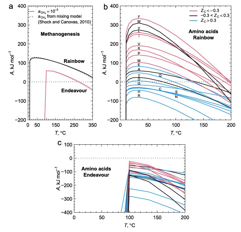
Figure 2. a. CH4 production releases more energy at the Rainbow hot vent field with ultramafic geology compared to the mafic Endeavour field when the hot fluids at the event are mixed with cold 2C seawater in greater amounts to reduce the temperature. b. The energetics of amino acid formation at Rainbow. More than half the amino acids are energetically favored. c. All amino acids are not energetically favored at Endeavour primarily due to the much lower molar H2 concentrations at Endeavour.

Figure 2b shows that some amino acids release energy when hot 350C water with reactants from Rainbow vents is mixed with cold seawater (approximately 6-10x dilution), while others require energy. The low H2 concentration in samples from Endeavour vents, about 25x more dilute, accounts for the negative affinities across all mixing temperatures at Endeavour. Why might this difference in the affinities between amino acids exist? One explanation is shown in figure 3a, that shows the oxidation values (Zc) of the amino acids. [Zc is a function of the oxidizing elements, charge, and is normalized by the number of carbon atoms of each amino acid. This sets a range of values as [-1.0,1.0].] Notably, those more energetically favored in figure 2b are also those that tend to be least oxidized, that is, they are mostly non-polar, hydrophobic amino acids with C-H bonds dominating.

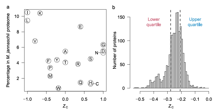
Figure 3. a. The oxidation level of amino acids. The higher the Zc value, the greater the number of oxidizing and polar atoms composing the amino acid. b. Histogram of all the proteins in the archaean Methanocaldococcus jannaschii based on their per amino acid carbons oxidation score.

Figure 3b shows the distribution of the Zc scores for the proteins of the archaean Methanocaldococcus jannaschii that is found in samples from Rainbow field. The distribution is notably skewed towards the more reduced proteins. The authors imply that this may be associated with the amino acids that have higher affinities and therefore their energy release of formation can be exploited by M. jannaschii.

The paper shows that all the organism’s proteins with their varying amino acid sequences have positive affinities from 0C to nearly 100C. As M. jannaschii has a preferred growth temperature of 85C, its whole protein production produces a net energy gain rather than requiring energy at this vent field, but would not have this energetic advantage if living at Endeavour. While M. jannaschii has an optimum growth temperature of 85C, one might expect other methanogens with optimal growth at lower temperatures closer to those of the optimal affinity values would have a competitive advantage.

As the authors state:

“Keeping in mind that temperature and composition are explicitly linked, these results show that the conditions generated during fluid mixing at ultramafic-hosted submarine hydrothermal systems are highly conducive to the formation of all of the proteins used by M. jannaschii.”

As the archaea already exploit the energetics of methane formation, do they also exploit the favorability of certain amino acids in the composition of their proteins, which are also favored energetically as the peptide bonds are formed?

While figure 3b is an interesting observation for one archaean species found at Rainbow, a natural question to ask is whether the different energetic favorability of certain amino acids is exploited by organisms at the vents by biasing the amino acid sequence of their proteomes, or whether this distribution is common across similar organisms both hot vent-living and surface-living organisms of methanogen archaea and other types of bacteria.

To put the M. jannaschii proteome Zc distribution in context, I have extended the authors’ analysis to other archaea and bacteria, living in hot vents, hypersaline, and constant mild temperature environments. Figure 4 shows the proteome Zc score distribution for 9 organisms. The black distributions are for the archaeans, and the red distributions for bacteria. The distributions for M. jannaschii and the model gut-living bacterium Escherichia coli are bolded.

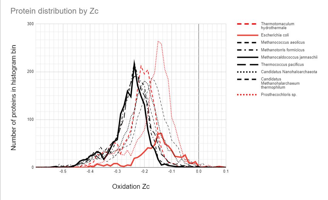
Figure 4. Histogram of proteome oxidation for various archaea (black) and bacteria (red). Several archaea living in hot temperatures are clustered together. The anaerobic, gut-living E. coli has a very different distribution. The bacterium Prosthecochloris that also lives in the hot vents has a distribution more similar to E. coli, whilst the hot vent living T. hydrothermale has a distribution between the vent-living archaea and E. coli. Two of the archaea also have distributions that deviate from the vent archaeans, one of which is adapted to the hot, hypersaline volcanic pools on the surface. (source author, Alex Tolley)

Figure 4 suggests that the explanation is more complex than simply the energetics as reflected in the proteome’s amino acid composition.

Firstly, the proteome distributions of M. jannaschii and E. coli are very different. They represent different domains of life, inhabit very different environments, and only M. jannaschii is a methanogen. So we have a number of different variables to consider.

Several archaea, all methanogens living in vents at different preferred temperatures, have similar proteome Zc score distributions. The two hypersaline archaea, Canditatus sp., have their distributions biased towards higher Zc scores that may reflect proteomes that are evolved to handle high salt concentrations. One is likely a methanogen, yet its distribution is further biased to a higher Zc score than the other. Of the bacteria, the hot vent-living Thermotomaculum hydrothermale has a Zc score distribution between E. coli and the similar archaean group. It is not a methanogen, but possibly it exploits the amino acid affinities of the hot vent environment.

The other vent-living bacterium, Prosthecochloris sp., has a distribution like that of E. coli. It is a photosynthesizing bacteria similar to green sulfur bacteria, and extracts geothermal light energy. It is not a methanogen. It is found in the sulfur rich smoker vents of the East Pacific Rise.

There seems to be two main possible explanations for the proteomic Zc distributions. Firstly, it may be due to a bias in the selection of amino acids that could release energy when in the H2-rich Rainbow habitat. Secondly, it could be the types of protein secondary structures that are needed for methanogenesis, so that structural reasons are the cause.

Figure 5 shows the protein structures for three approximately matching Zc scores and sequence length for M. jannaschii and E. coli. What stands out is that the lower the Zc score, the more the alpha-helix secondary structure appears in the protein tertiary structure. Both organisms appear to have similar secondary structure compositions when the Zc scores are matched, suggesting that the distribution differences are due to the numbers of proteins with alpha-helix structures rather than some fundamental difference in the sequences. Is this a clue to the underlying distribution?

The amino acids that principally appear in helices are the “MALEK” set, methionine, alanine, leucine, glutamic acid and lysine [6]. A helix made up of equal amounts of each of these amino acids has a Zc score of -0.4, all coincidently in the positive affinity range of amino acids in Rainbow, as shown in figure 2b. This is highly suggestive that the reason for the different distributions is a bias in the production of proteins that have an abundance of alpha-helix secondary structures.

Figure 5. Comparison of selected proteins from M. jannaschii and E. coli spanning the range of Zc scores.

Which proteins might be those with sequences that have higher high alpha-helix structures? As a distinguishing feature of archaea is methanogenesis, a good start is to look at the proteins involved in methane metabolism.

Figure 6 shows the methanogenesis pathways of methane metabolism highlighted. The genes associated with the methanogenesis annotated proteins of M. jannaschii are boxed in blue and are mostly connected with the early CO2 metabolism. From this, some proteins were selected that had tertiary structure available to be viewed in the Uniprot database [3].

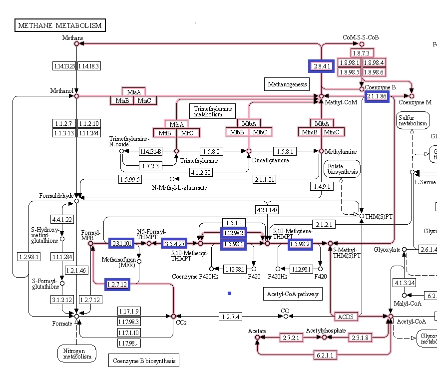
Figure 6. Methane metabolism pathway highlighted. Source: Kegg database [4].

Figure 7. Selected proteins from the methane metabolism pathway of archaea showing the predominance of helix structures [The Kegg #.#.#.# identifiers are shown to map to figure 5.].

The paucity of good, available tertiary protein structures for the methanogenesis pathways makes the selection support a more anecdotal than analytic explanation. The selected proteins do suggest that they are highly composed of alpha-helices. If the methanogenesis pathways are more highly populated with proteins with helical structures, then the explanation of the hot vent-living archaeans might hold.

In other words, it is not, particularly the energetic favorability that determines the proteome composition, but rather the types of metabolic pathways, most likely methanogenesis that is responsible. It should be noted that pathway proteins are not populated by one unique protein as the Kegg pathway indicates where several closely related genes/proteins can be involved in the same function.

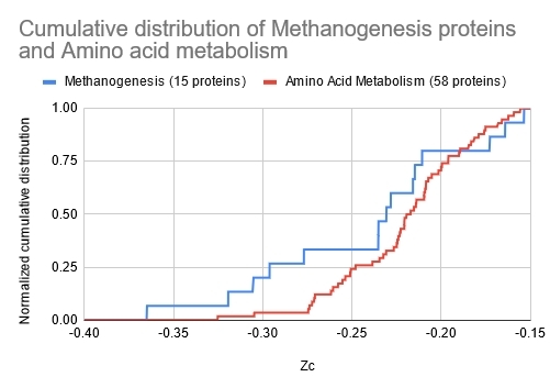
Figure 8. Cumulative distribution of proteins for methanogenesis and amino acid metabolism for M. jannaschii. The methanogenesis proteins are biased towards the lower Zc values, indicating a greater probability of alpha-helix structures.

Figure 7 shows the normalized cumulative distributions of 15 methanogenesis proteins and 58 amino acid metabolizing proteins that have been well identified for M. jannashii.

The distribution clearly shows that there is a bias towards the lower Zc values for the methanogenesis proteins than the more widely distributed amino acid metabolic proteins. While not definitive, it is suggestive that the proteome Zc score distribution between organisms may be accounted for by the presence and numbers of methanogenesis proteins.

Lastly, I want to touch on some speculation on the larger question of abiogenesis. It is unclear whether bacteria or archaea are the older life forms and closer to the last universal common ancestor (LUCA). Because the archaea share some similarities to the eukaryotes, this implies that either the bacteria are the earlier form, or that they are a later form that branched off from the archaea, and the eukaryotes evolved from the archaean branch. The attractiveness of the archaea as the most ancestral forms, as their domain name suggests, is their extremophile nature and their ability to extract energy from the geologic production of H2 to form CH4 as autotrophs, rather than consuming CH4, which has been shown to be relatively out of equilibrium due to the energy barrier to complete the reaction.

If so, does the energetic favorability of amino acid formation at ultramafic hot vent locations suggest a possible route to abiogenesis via a metabolism first model? While the reaction to create amino acids abiotically may be difficult to proceed, they may accumulate over time as long as the reverse reactions to degrade them are largely absent. As peptide bonds are energetically favored, oligopeptides and proteins could form abiotically at the vents as the hot fluids mix with the cold ocean water.

If so, could random small proteins form autocatalytic sets that lead to metabolism and reproduction? A number of experiments indicate that amino acids will spontaneously link together and that they can be autocatalytic for self-replication. Peptides replacing the sugar-phosphate backbone can link nucleobases that also can replicate, the model that was held to be a feature of the RNA World model.

But there is a potential fly in the ointment of this explanation of abiogenic protein formation. The proteins should be formed from amino acids that are composed of both L and D chiral forms. Life has selected one form and is homochiral, a feature that is suggested as a determinant for the origin of any extraterrestrial biologically important molecules detected. Experiments have suggested that any small bias in chirality, due perhaps to the crystal surface structure of the rocks, can lead to an exponential dominance of one chiral form over the other. Ribo et al published a review of this spontaneous mirror symmetry breaking (SMSB) [5].

So we have a possible model of abiotically formed peptides of random amino acid sequences that collect in the pores of rocks at the vents and may be surrounded by lipid membranes. The proteins can both form metabolic pathways and self replicate. If the peptides mostly form self-replicating helices, and these can be co-opted to further extract energy via methanogenesis, then we have a possible model for the emergence of life.

As my earlier article speculated that radiolysis could ensure that chemotrophs in the crust of a wide variety of planets and moons could be supported, we can now speculate that the favorable energetics of amino acid and protein formation may also drive the emergence of life.

As autotrophic organisms like archaea can evolve to exploit the energetics of CH4 and protein production under favorable conditions at seafloor vents, and support the evolving ecosystems of chemotrophs, this suggests that abiotic reactions may have started the process that evolved into the sophisticated methanogenesis pathways of methanogens we see today.

If correct, then life may be common in the galaxy wherever the conditions are right, that is that where ultramafic rocks in the mantle, heated from below by various means, and in contact with cold ocean water exist in combination, whether on a planet similar to the early Earth or possibly at the boundary of the mantle and the deep subsurface oceans of icy moons outside the bounds of the traditional habitable zone.

References

Tolley, A “Radiolytic H2: Powering Subsurface Biospheres” (2021) URL accessed 12/01/2021:
https://www.centauri-dreams.org/2021/07/02/radiolytic-h2-powering-subsurface-biospheres/

Dick, J, Shock, E. “The Release of Energy During Protein Synthesis at Ultramafic-Hosted Submarine Hydrothermal Ecosystems” (2021) JournalJournal of Geophysical Research: Biogeosciences, v126:11.
https://agupubs.onlinelibrary.wiley.com/doi/full/10.1029/2021JG006436

Uniprot database
uniprot.org

Kegg database
genome.jp/kegg/

Ribo, J et al “Spontaneous mirror symmetry breaking and origin of biological homochirality” (2017) Journal of the Royal Society Interface, v14:137
https://royalsocietypublishing.org/doi/10.1098/rsif.2017.0699

Alpha-Helix
https://en.wikipedia.org/wiki/Alpha_helix

The ‘Disintegrating Planet’ Factor

Using machine learning to provide an algorithmic approach to the abundant data generated by the Transiting Exoplanet Survey Satellite (TESS) has proven unusually productive. I’m looking at an odd object called TIC 400799224, as described in a new paper in The Astronomical Journal from Brian Powell (NASA GSFC) and team, a source that displays a sudden drop in brightness – 25% in a matter of four hours – followed by a series of brightness variations. What’s going on here?

We’re looking at something that will have to be added to a small catalog of orbiting objects that emit dust; seven of these are presented in the paper, including this latest one. The first to turn up was KIC 12557548, whose discovery paper in 2012 argued that the object was a disintegrating planet emitting a dust cloud, a model that was improved in subsequent analyses. K2-22b, discovered in 2015, showed similar features, with varying transit depths and shapes, although no signs of gas absorption..

In fact, the objects in what we can call our ‘disintegrating planet catalog’ are rather fascinating. WD 1145+017 is a white dwarf evidently showing evidence for orbiting bodies emitting dust, with masses of each found to be comparable to our Moon. These appear to be concentrations of dust rather than solid bodies. And another find, ZTF J0139+5245, may turn out to be a white dwarf orbited by extensive planetary debris.

So TIC 400799224 isn’t entirely unusual in showing variable transit depths and durations, a possibly disintegrating body whose transits may or may not occur when expected. But dig deeper and, the authors argue, this object may be in a category of its own. This is a widely separated binary system, the stars approximately 300 AU apart, and at this point it is not clear which of the two stars is the host to the flux variations. The light curve dips are found only in one out of every three to five transits.

All of this makes it likely that what is occulting the star is some kind of dust cloud. Studying the TESS data and following up with a variety of ground-based instruments, the authors make the case: One of the stars is pulsating with a 19.77 day period that is probably the result of an orbiting body emitting clouds of dust. The dust cloud involved is substantial enough to block between 37% and 75% of the star’s light, depending on which of the two stars is the host. But while the quantity of dust emitted is large, the periodicity of the dips has remained the same over six years of observation.

Image: An optical/near-infrared image of the sky around the TESS Input Catalog (TIC) object TIC 400799224 (the crosshair marks the location of the object, and the width of the field of view is given in arcminutes). Astronomers have concluded that the mysterious periodic variations in the light from this object are caused by an orbiting body that periodically emits clouds of dust that occult the star. Credit: Powell et al., 2021.

How is this object producing so much dust, and how does it remain intact, with no apparent variation in periodicity? The authors consider sublimation as a possibility but find that it doesn’t replicate the mass loss rate found in TIC 400799224. Also possible: A ‘shepherding’ planet embedded within the dust, although here we would expect more consistent light curves from one transit to the next. Far more likely is a series of collisions with a minor planet. Let me quote the paper on this:

A long-term (at least years) phase coherence in the dips requires a principal body that is undergoing collisions with minor bodies, i.e., ones that (i) do not destroy it, and (ii) do not even change its basic orbital period. The collisions must be fairly regular (at least 20–30 over the last 6 years) and occur at the same orbital phase of the principal body.

This scenario emerges, in the authors’ estimate, as the most likely:

Consider, for example, that there is a 100 km asteroid in a 20 day orbit around TIC 400799224. Further suppose there are numerous other substantial, but smaller (e.g., ≲1/10th the radius), asteroids in near and crossing orbits. Perhaps this condition was set up in the first place by a massive collision between two larger bodies. Once there has been such a collision, all the debris returns on the next orbit to nearly the same region in space. This high concentration of bodies naturally leads to subsequent collisions at the same orbital phase. Each subsequent collision produces a debris cloud, presumably containing considerable dust and small particles, which expands and contracts vertically, while spreading azimuthally, as time goes on. This may be sufficient to make one or two dusty transits before the cloud spreads and dissipates. A new collision is then required to make a new dusty transit.

Amateur astronomers may want to see what they can learn about this object themselves. The authors point out that it’s bright enough to be monitored by ‘modest-size backyard telescopes,’ allowing suitably equipped home observers to look for transits. Such transits should also show up in historical data, giving us further insights into the behavior of the binary and the dust cloud producing this remarkably consistent variation in flux. As noted, the object in question evidently remains intact.

Digression: I mentioned earlier how much machine learning has helped our analysis of TESS data. The paper makes this clear, citing beyond TIC 400799224 such finds as:

several hundred thousand eclipsing binaries in TESS light curves;a confirmed sextuple star system;a confirmed quadruple star system;many additional quadruple star system candidates;numerous triple star system candidates;“candidates for higher-order systems that are currently under investigation.”

Algorithmic approaches to light curves are becoming an increasingly valuable part of the exoplanet toolkit, about which we’ll be hearing a great deal more.

The paper is Powell et al, “Mysterious Dust-emitting Object Orbiting TIC 400799224,” The Astronomical Journal Vol. 162, No. 6 (8 December 2021). Full text.

Rogue Planet Discoveries Challenge Formation Models

As we begin the New Year, I want to be sure to catch up with the recent announcement of a discovery regarding ‘rogue’ planets, those interesting worlds that orbit no central star but wander through interstellar space alone (or, conceivably, with moons). Conceivably ejected from their host stars through gravitational interactions (more on this in a moment), such planets become interstellar targets in their own right, as given the numbers now being suggested, there may be rogue planets near the Solar System.

Image: Rogue planets are elusive cosmic objects that have masses comparable to those of the planets in our Solar System but do not orbit a star, instead roaming freely on their own. Not many were known until now, but a team of astronomers, using data from several European Southern Observatory (ESO) telescopes and other facilities, have just discovered at least 70 new rogue planets in our galaxy. This is the largest group of rogue planets ever discovered, an important step towards understanding the origins and features of these mysterious galactic nomads. Credit: /ESO/COSMIC-DANCE Team/CFHT/Coelum/Gaia/DPAC.

A brief digression on the word ‘interstellar’ in this context. I consider any mission outside the heliosphere to be interstellar, in that it takes the spacecraft into the interstellar medium. Our two Voyagers are in interstellar space – hence NASA’s monicker Voyager Interstellar Mission – even if not designed for it. The Sun’s gravitational influence extends much further, as the Oort Cloud attests, but the heliosphere marks a useful boundary, one that contains the solar wind within. The great goal, a mission from one star to another, is obviously the ultimate interstellar leap.

How many rogue planets may be passing through our galactic neighborhood? Without a star to illuminate them, they can and have been searched for via microlensing signatures. But the new work, in the hands of Hervé Bouy (Laboratoire d’Astrophysique de Bordeaux), uses data not just from the Very Large Telescope but other instruments in Chile including the adjacent VISTA (Visible and Infrared Survey Telescope for Astronomy), the VLT Survey Telescope and the MPG/ESO 2.2-metre telescope.

Tens of thousands of wide-field images went into the survey. The target: A star-forming region close to the Sun in the constellations Scorpius and Ophiuchus. The work takes advantage of the fact that planets that are young enough continue to glow brightly in the infrared, allowing us to go beyond microlensing methods to find them. About 70 potential rogue planets turn up in this survey. Núria Miret-Roig (Laboratoire d’Astrophysique de Bordeaux), first author of the paper on this work, comments:

“We measured the tiny motions, the colours and luminosities of tens of millions of sources in a large area of the sky. These measurements allowed us to securely identify the faintest objects in this region, the rogue planets…There could be several billions of these free-floating giant planets roaming freely in the Milky Way without a host star.”

Image: The locations of 115 potential FFPs [free-floating planets] in the direction of the Upper Scorpius and Ophiuchus constellations, highlighted with red circles. The exact number of rogue planets found by the team is between 70 and 170, depending on the age assumed for the study region. This image was created assuming an intermediate age, resulting in a number of planet candidates in between the two extremes of the study. Credit: ESO/N. Risinger (skysurvey.org).

But we need to pause on the issue of stellar age. What these measurements lack is the ability to determine the mass of the discovered objects. Without that, we have problems distinguishing between brown dwarf stars – above 13 Jupiter masses – and planets. What Miret-Roig’s team did was to rely on the brightness of the objects in order to set upper limits on their numbers. Brightness varies with age, so that in older regions, brighter objects are likely above 13 Jupiter masses, while in younger ones, they are assumed to be below that value. The value is uncertain enough in the region in question to yield between 70 and 170 rogue planets.

Planet formation is likewise an interesting question here. I mentioned ejection from planetary systems above, but these free-floating planets are young enough to call that scenario into question. In fact, other mechanisms are discussed in the literature. The paper notes the possibility of core-collapse (a version of star formation), with the variant that a stellar embryo might be ejected from a star-forming nursery before building up sufficient mass to become a star. We need to build up our data on rogue planets to discover the relative contribution of each method to the population.

This work uncovers more rogue planets by a factor of seven than core-collapse models predict, making it likely that other methods are at work:

This excess of FFPs [free-floating planets] with respect to a log-normal mass distribution is in good agreement with the results reported in σ Orionis [a multiple system that is a member of an open cluster in Orion]. Interestingly, our observational mass function also has an excess of low-mass brown dwarfs and FFPs with respect to simulations including both core-collapse and disc fragmentation . This suggests that some of the FFPs in our sample could have formed via fast core-accretion in discs rather than disc fragmentation. We also note that the continuity of the shape of the mass function at the brown dwarf/planetary mass transition suggests a continuity in the formation mechanisms at work for these two classes of objects.

So the formation of rogue planets is considerably more complicated than I made it appear in my opening paragraph. The authors believe that ejection from planetary systems is roughly comparable to core-collapse as a planet formation model. That would imply that dynamical instabilities in exoplanet systems (at least, those containing gas giants) produce ejections frequently within the first 10 million years after formation. Investigating these extremely faint objects further will require the capabilities of future instrumentation like the Extremely Large Telescope.

The paper is Miret-Roig et al, “A rich population of free-floating planets in the Upper Scorpius young stellar association,” published online at Nature Astronomy 22 December 2021 (abstract).

The Goodness of the Universe

The end of one year and the beginning of the next seems like a good time to back out to the big picture. The really big picture, where cosmology interacts with metaphysics. Thus today’s discussion of evolution and development in a cosmic context. John Smart wrote me after the recent death of Russian astronomer Alexander Zaitsev, having been with Sasha at the 2010 conference I discussed in my remembrance of Zaitsev. We also turned out to connect through the work of Clément Vidal, whose book The Beginning and the End tackles meaning from the cosmological perspective (see The Zen of SETI). As you’ll see, Smart and Vidal now work together on concepts described below, one of whose startling implications is that a tendency toward ethics and empathy may be a natural outgrowth of networked intelligence. Is our future invariably post-biological, and does such an outcome enhance or preclude journeys to the stars? John Smart is a global futurist, and a scholar of foresight process, science and technology, life sciences, and complex systems. His book Evolution, Development and Complexity: Multiscale Evolutionary Models of Complex Adaptive Systems (Springer) appeared in 2019. His latest title, Introduction to Foresight, 2021, is likewise available on Amazon.

by John Smart

In 2010, physicists Martin Dominik and John Zarnecki ran a Royal Society conference, Towards a Scientific and Societal Agenda on Extra-Terrestrial Life addressing scientific, legal, ethical, and political issues around the search for extra-terrestrial intelligence (SETI). Philosopher Clement Vidal and I both spoke at that conference. It was the first academic venue where I presented my Transcension Hypothesis, the idea that advanced intelligence everywhere may be developmentally-fated to venture into inner space, into increasingly local and miniaturized domains, with ever-greater density and interiority (simulation capacity, feelings, consciousness), rather than to expand into “outer space”, the more complex it becomes. When this process is taken to its physical limit, we get black-hole-like domains, which a few astrophysicists have speculated may allow us to “instantly” connect with all the other advanced civilizations which have entered a similar domain. Presumably each of these intelligent civilizations will then compare and contrast our locally unique, finite and incomplete science, experiences and wisdom, and if we are lucky, go on to make something even more complex and adaptive (a new network? a universe?) in the next cycle.

Clement and I co-founded our Evo-Devo Universe complexity research and discussion community in 2008 to explore the nature of our universe and its subsystems. Just as there are both evolutionary and developmental processes operating in living systems, with evolutionary processes being experimental, divergent, and unpredictable, and developmental processes being conservative, convergent, and predictable, we think that both evo and devo processes operate in our universe as well. If our universe is a replicating system, as several cosmologists believe, and if it exists in some larger environment, aka, the multiverse, it is plausible that both evolutionary and developmental processes would self-organize, under selection, to be of use to the universe as complex system. With respect to universal intelligence, it seems reasonable that both evolutionary diversity, with many unique local intelligences, and developmental convergence, with all such intelligences going through predictable hierarchical emergences and a life cycle, would emerge, just as both evolutionary and developmental processes regulate all living intelligences.

Once we grant that developmental processes exist, we can ask what kind of convergences might we predict for all advanced civilizations. One of those processes, accelerating change, seems particularly obvious, even though we still don’t have a science of that acceleration. (In 2003 I started a small nonprofit, ASF, to make that case). But what else might we expect? Does surviving universal intelligence become increasingly good, on average? Is there an “arc of progress” for the universe itself?

Developmental processes become increasingly regulated, predictable, and stable as function of their complexity and developmental history. Think of how much more predictable an adult organism is than a youth (try to predict your young kids thinking or behavior!), or how many less developmental failures occur in an adult versus a newly fertilized embryo. Development uses local chaos and contingency to converge predictably on a large set of far-future forms and functions, including youth, maturity, replication, senescence, and death, so the next generation may best continue the journey. At its core, life has never been about either individual or group success. Instead, life’s processes have self-organized, under selection, to advance network success. Well-built networks, not individuals or even groups, always progress. As a network, life is immortal, increasingly diverse and complex, and always improving its stability, resiliency, and intelligence.

But does universal intelligence also become increasingly good, on average, at the leading edge of network complexity? We humans are increasingly able to use our accelerating S&T to create evil, with ever-rising scale and intensity. But are we increasingly free to do so, or do we grow ever-more self-regulated and societally constrained? Steven Pinker, Rutger Bregman, and many others argue we have become increasingly self- and socially-constrained toward the good, for yet-unclear reasons, over our history. Read The Better Angels of Our Nature, 2012 and Humankind, 2021 for two influential books on that thesis. My own view on why we are increasingly constrained to be good is because there is a largely hidden but ever-growing network ethics and empathy holding human civilizations together. The subtlety, power, and value of our ethics and empathy grows incessantly in leading networks, apparently as a direct function of their complexity.

As a species, we are often unforesighted, coercive, and destructive. Individually, far too many of us are power-, possession- or wealth-oriented, zero-sum, cruel, selfish, and wasteful. Not seeing and valuing the big picture, we have created many new problems of progress, like climate change and environmental destruction, that we shamefully neglect. Yet we are also constantly progressing, always striving for positive visions of human empowerment, while imagining dystopias that we must prevent.

Ada Palmer’s science fiction debut, Too Like the Lightning, 2017 (I do not recommend the rest of the series), is a future world of technological abundance, accompanied by dehumanizing, centrally-planned control over what individuals can say, do, or believe. I don’t think Palmer has written a probable future. But it is plausible, under the wrong series of unfortunate and unforesighted future events, decisions and actions. Imagining such dystopias, and asking ourselves how to prevent them, is surely as important as positive visions to improving adaptiveness. I am also convinced we are rapidly and mostly unconsciously creating a civilization that will be ever more organized around our increasingly life-like machines. We can already see that these machines will be far smarter, faster, more capable, more miniaturized, more resource-independent, and more sustainable than our biology. That fast-approaching future will be importantly different from (and better than?) anything Earth’s amazing, nurturing environment has developed to date, and it is not well-represented in science-fiction yet, in my view.

On average, then, I strongly believe our human and technological networks grow increasingly good, the longer we survive, as some real function of their complexity. I also believe that postbiological life is an inevitable development, on all the presumably ubiquitous Earthlike planets in our universe. Not only does it seem likely that we will increasingly choose to merge with such life, it seems likely that it will be far smarter, stabler, more capable, more ethical, empathic, and more self-constrained than biological life could ever be, as an adaptive network. There is little science today to prove or disprove such beliefs. But they are worth stating and arguing.

Arguing the goodness of advanced intelligence was the subtext of the main debate at the SETI conference mentioned above. The highlight of this event was a panel debate on whether it is a good idea to not only listen for signs of extraterrrestrial intelligence (SETI), but to send messages (METI), broadcasting our existence, and hopefully, increase the chance that other advanced intelligences will communicate with us earlier, rather than later.

One of the most forceful proponents for such METI, Alexander Zaitsev, spoke at this conference. Clement and I had some good chats with him there (see picture below). Since 1999, Zaitsev has been using a radiotelescope in the Ukraine, RT-70, to broadcast “Hello” messages to nearby interesting stars. He did not ask permission, or consult with many others, before sending these messages. He simply acted on his belief that doing so would be a good act, and that those able to receive them would not only be more advanced, but would be inherently more good (ethical, empathic) than us.

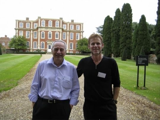
Image: Alexander Zaitsev and John Smart, Royal Society SETI Conference, Chicheley Hall, UK, 2010. Credit: John Smart.

Sadly, Zaitsev has now passed away (see Paul Gilster’s beautiful elegy for him in these pages). It explains the 2010 conference, where Zaitsev debated others on the METI question, including David Brin. Brin advocates the most helpful position, one that asks for international and interdisciplinary debate prior to sending of messages. Such debate, and any guidelines it might lead to, can only help us with these important and long-neglected questions.

It was great listening to these titans debate at the conference, yet I also realized how far we are from a science that tells us the general Goodness of the Universe, to validate Zaitsev’s belief. We are a long way from his views being popular, or even discussed, today. Many scientists assume that we live in a randomness-dominated, “evolutionary” universe, when it seems much more likely that it is an evo-devo universe, with both many unpredictable and predictable things we can say about the nature of advanced complexity. Also, far too many of us still believe we are headed for the stars, when our history to date shows that the most complex networks are always headed inward, into zones of ever-greater locality, miniaturization, complexity, consciousness, ethics, empathy, and adaptiveness. As I say in my books, it seems that our destiny is density, and dematerialization. Perhaps all of this will even be proven in some future network science. We shall see.

Remote Observation: What Could ET See?

As we puzzle out the best observing strategies to pick up a bio- or technosignature, we’re also asking in what ways our own world could be observed by another civilization. If such exist, they would have a number of tools at their disposal by which to infer our existence and probe what we do. Extrapolation is dicey, but we naturally begin with what we understand today, as Brian McConnell does in this, the third of a three-part series on SETI issues. A communications systems engineer, Brian has worked with Alex Tolley to describe a low-cost, high-efficiency spacecraft in their book A Design for a Reusable Water-based Spacecraft Known as the Spacecoach (Springer, 2015). His latest book is The Alien Communication Handbook — So We Received A Signal, Now What? recently published by Springer Nature. Is our existence so obvious to the properly advanced observer? That doubtless depends on the state of their technology, about which we know nothing, but if the galaxy includes billion-year old cultures, it’s hard to see how we might be missed.

by Brian McConnell

In SETI discussions, it is often assumed that an ET civilization would be unaware of our existence until they receive a signal from us. I Love Lucy is an often cited example of early broadcasts they might stumble across. Just as we are developing the capability to directly image exoplanets, a more astronomically advanced civilization may already be aware of our existence, and may have been for a long time. Let’s consider several methods by which an ET could take observations of Earth:

Spectroscopic analysis of Earth’s atmosphereDeconvolution of Earth’s light curveSolar gravitational lens telescopesSolar system scale interferometersHigh speed flyby probes (e.g. Starshot)Slow traveling probes that loiter in near Earth space (Lurkers, Bracewell probes)Spectroscopic Analysis

We are already capable of conducting spectroscopic analysis of the light passing through exoplanet atmospheres, and as a result, are able to learn about their general characteristics. This capability will soon be extended to include Earth sized planets. An ET astronomer that had been studying Earth’s atmosphere over the past several centuries would have been able to see the rapid accumulation of carbon dioxide and other fossil fuel waste gases. This signal is plainly evident from the mid 1800s onward. Would this be a definitive sign of an emergent civilization? Probably not, but it would be among the possible explanations, and perhaps a common pattern as an industrial civilization develops. Other gases, such as fluorocarbons (CFCs and HFCs) have no known natural origin, and would more clearly indicate more recent industrial activity.

There is also no reason not to stop at optical/IR, and not conduct similar observations in the microwave band, both to look for artificial signals such as radars, but also to study the magnetic environment of exoplanets, much like we are using the VLA to study the magnetic fields of exoplanets. It’s worth noting that most of the signals we transmit are not focused at other star systems, and would appear very weak to a distant observer, though they might notice a general brightening in the microwave spectrum, much like artificial illumination might be detectable. This would be a sure sign of intelligence, but we have not been “radio bright” for very long, so this would only be visible to nearby systems.

Deconvolution

Even if we can only obtain a single pixel image of an exoplanet, we can use a technique called deconvolution to develop a low resolution image of it by measuring how its brightness and color varies as the planet rotates. This is not unlike building an image by moving a light meter across a surface to build a map of light levels that can be translated into an image. It won’t be possible to build a high resolution image, but it will be possible to see large-scale features such as oceans, continents and ice caps. While it would not be possible to directly see human built structures, it would be clear that Earth has oceans and vegetation. Images of Pluto taken before the arrival of the New Horizons probe offer an example of what can be done with a limited amount of information.

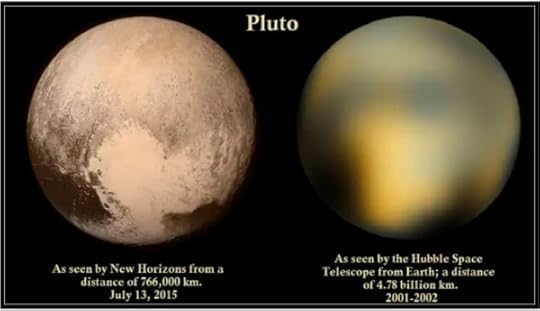
Comparison of images of Pluto taken by the New Horizons probe (left) and the Hubble Space Telescope via light curve reconstruction (right). Image credit: NASA / Planetary Society.

Svetlana Berdyugina and Jeff Kuhn presented a presentation on this topic at the 2018 NASA Techno Signatures symposium where they simulated what the Earth would look like through this deconvolution process. In the simulated image, continents, oceans and ice caps are clearly visible, and because the Earth’s light curve can be split out by wavelength, it would be possible to see evidence of vegetation.

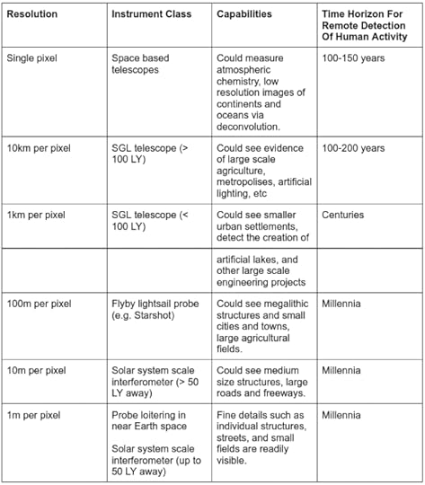
Solar Gravitational Lens Telescopes

A telescope placed along a star’s gravitational lens focal line will be able to take multi pixel images of exoplanets at considerable distances. Slava Turyshev et al show in this NASA NIAC paper that it will be possible to use an SGL telescope to image exoplanets at 1 kilometer per pixel resolution out to distances of 100 light years. A SGL telescope pointed at Earth might be able to see evidence of large scale agriculture, urban centers, night side illumination, reservoirs, and other signs of civilization. Moreover, pre-industrial activity and urban settlements might be visible to this type of instrument, which raises the possibility that an ET civilization with this capability would have been able to see evidence of human civilization centuries ago, perhaps Longer.

A simulated image of an exoplanet as seen from an SGL telescope. Image credit: NASA/JPL

A spacefaring civilization that happens to have access to a nearby black hole would have an even better lens to use (the Sun’s gravitational lens is slightly distorted because of the Sun’s rotation and oblate shape).

Solar System Scale Interferometers

The spatial resolution of a telescope is a function of its aperture size and the wavelength of the light being observed. Using interferometry, widely separated telescopes can combine their observations, and increase the effective aperture to the distance between the telescopes. The Black Hole Event Horizon Telescope used interferometry to create a virtual radio telescope whose aperture was the size of Earth. With it, we were able to directly image the accretion disc of galaxy M87’s central black hole, some 53 million light years away.

Synthetic microwave band image of M87’s central black hole’s shadow and nearby environment. Image credit: Event Horizon Telescope

Now imagine a fleet of optical interferometers in orbit around a star. They would have an effective aperture measuring tens to hundreds of millions of kilometers, and would be able to see small surface details on distant exoplanets. This is beyond our capabilities to build today, but the underlying physics say they will be possible to build, which is to say it is an expensive and difficult engineering problem, something a more advanced civilization may have built. Indeed, we began to venture down this path with the since canceled SIM (Space Interferometry Mission) and LISA (Laser Interferometer Space Antenna) telescopes.

A solar system scale constellation of optical interferometers would be able to resolve surface details of distant objects at a resolution of 1-10 meters per pixel, comparable to satellite imagery of the Earth, meaning that even early agriculture and settlements would be visible to them.

Fast Flyby Probes

Fast lightsail probes, similar to the Breakthrough Starshot probes that we hope to fly in a few decades, will be able to take high resolution images of exoplanets as the probes fly past target planets. Images taken of Pluto by the New Horizons probe probably give an idea of what to expect in terms of resolution. It was able to return images at a resolution of less than 100 meters per pixel, smaller than a city block.

The primary challenges in obtaining high resolution images from probes like these are: the speed at which the probe flies past its target (0.2c in the case of the proposed starshot probe),and transmitting observations back to the home system. Both of these are engineering problems. For example, the challenge of capturing images can be solved by taking as many images as possible during the flyby and then using on board post processing to create a synthesized image. Communication is likewise an engineering problem that can be solved with better onboard power sources and/or large receiving facilities at the home system. If the probe itself is autonomous and somewhat intelligent, it can also decide which parts of the collected imagery are most interesting and prioritize their transmission.

The Breakthrough Starshot program envisions launching a large number of cheap, lightweight lightsails on a regular cadence, so while an individual probe might only be able to capture a limited set of observations, in aggregate they may be able to return extensive observations and imagery over an extended period of time.

Slow Loitering Probes (Lurkers and Bracewell Probes)

An ET civilization that has worked out nuclear propulsion would be able to send slower traveling probes to loiter in near Earth space. These probes could be long lived, and could be designed for a variety of purposes. Being in close proximity to Earth, they would be able to take high resolution images over an extended period of time. Consider that the Voyager probes, among the first deep space probes we built, are still operational today. ET probes could be considerably more long lived and capable of autonomous operation. If they are operating in our vicinity, they would have been able to see early signs of human activity back to antiquity. One important limitation is that only nearby civilizations would be able to launch probes to our vicinity within a few hundred years.

The implication of this is not just that an ETI could be able to see us today, they could have been able to study the development of human civilization from afar, over a period spanning centuries or millennia. Beyond that, Earth has had life for 3.5 billion years, and life on land for several hundred million years. So if other civilizations are surveying habitable worlds on an ongoing basis, Earth may have been noticed and flagged as a site of interest long before we appeared on the scene.

One of the criticisms of SETI is that the odds of two civilizations going “online” within an overlapping time frame may be vanishingly small, which implies that searching for signals from other civilizations may be a lost cause. But what if early human engineering projects, such as the Pyramids of Giza, had been visible to them long ago? Then the sphere of detectability expands by orders of magnitude, and more importantly, these signals we have been broadcasting unintentionally have been persistent and visible for centuries or millennia.

This has ramifications for active SETI (METI) as well. Arguments against transmitting our own artificial signals, on the basis that we might be risking hostile action by neighbors, may be moot if most advanced civilizations have some of the capabilities mentioned in this article. At the very least, they would know Earth is an inhabited world and a site for closer study, and may well have been able to see early signs of human civilization long ago. So perhaps it is time to revisit the METI debate, but this time with a focus on understanding what unintentional signals or techno signatures we have been sending and who could see them.

A Holiday Check-in with New Horizons

The fact that we have three functioning spacecraft outside the orbit of Pluto fills me with holiday good spirits. Of the nearest of the three, I can say that since New Horizons’ January 1, 2019 encounter with the Kuiper Belt Object now known as Arrokoth, I have associated the spacecraft with holidays of one kind or another The July 14, 2015 flyby of Pluto/Charon wasn’t that far off the US national holiday, but more to the point, I was taking a rare beach vacation during the last of the approach phase, most of my time spent indoors with multiple computers open tracking events at system’s edge. It felt celebratory, like an extended July 4, even if the big event was days later.

Also timely as the turn of the year approaches is Alan Stern’s latest PI’s Perspective, a look at what’s ahead for the plucky spacecraft. Here January becomes a significant time, with the New Horizons team working on the proposal for another mission extension, the last of which got us through Arrokoth and humanity’s first close-up look at a KBO. The new proposal aims at continued operations from 2023 through 2025, which could well include another KBO flyby, if an appropriate target can be found. That search, employing new machine learning tools, continues.

Image: Among several discoveries made during its flyby of the Kuiper Belt object Arrokoth in January 2019, New Horizons observed the remarkable and enigmatic bright, symmetric, ring-like “neck” region at the junction between Arrokoth’s two massive lobes. Credit: NASA/Johns Hopkins APL/Southwest Research Institute.

But what happens if no KBO is within reach of the spacecraft? Stern explains why the proposed extension remains highly persuasive:

If a new flyby target is found, we will concentrate on that flyby. But if no target is found, we will convert New Horizons into a highly-productive observatory conducting planetary science, astrophysics and heliospheric observations that no other spacecraft can — simply because New Horizons is the only spacecraft in the Kuiper Belt and the Sun’s outer heliosphere, and far enough away to perform some unique kinds of astrophysics. Those studies would range from unique new astronomical observations of Uranus, Neptune and dwarf planets, to searches for free floating black holes and the local interstellar medium, along with new observations of the faint optical and ultraviolet light of extragalactic space. All of this, of course, depends on NASA’s peer review evaluation of our proposal.

Our only spacecraft in the Kuiper Belt. What a reminder of how precious this asset is, and how foolish it would be to stop using it! Here my natural optimism kicks in (admittedly beleaguered by the continuing Covid news, but determined to push forward anyway). One day – and I wouldn’t begin to predict when this will be – we’ll have numerous Kuiper Belt probes, probably enabled by beamed sail technologies in one form or another as we continue the exploration of the outer system, but for now, everything rides on New Horizons.

The ongoing analysis of what New Horizons found at Pluto/Charon is a reminder that no mission slams to a halt when one or another task is completed. For one thing, it takes a long time to get data back from New Horizons, and we learn from Stern’s report that a good deal of the flyby data from Arrokoth is still on the spacecraft’s digital recorders, remaining there because of higher-priority transmission needs as well as scheduling issues with the Deep Space Network. We can expect the flow of publications to continue. 49 new scientific papers came out this year alone.

That Arrokoth image above is still a stunner, and the inevitable naming process has begun not only here but on Pluto as well. The KBO’s largest crater has been christened ‘Sky,’ while Ride Rupes (for astronaut Sally Ride) and Coleman Mons (for early aviator Bessie Coleman) likewise will begin to appear on our maps of Pluto. All three names have been approved by the International Astronomical Union. ‘Rupes’ is the Latin word for ‘cliff,’ and here refers to an enormous feature near the southern tip of Pluto’s Tombaugh Regio. Ride Rupes is between 2 and 3 kilometers high and about 250 kilometers long, while Coleman Mons is a mountain, evidently recently created and thus distinctive in a region of older volcanic domes.

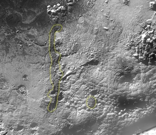
Image: Close-up, outlines of Ride Rupes (left) and Coleman Mons on the surface Pluto. Credit: NASA/Johns Hopkins APL/Southwest Research Institute/SETI Institute/Ross Beyer.

As the New Horizons team completes the mission extension proposal, it also proceeds with uploading another instrument software upgrade, this one to the Pluto Energetic Particle Spectrometer Science Investigation (PEPSSI) charged-particle spectrometer. And while spacecraft power levels have continued to decline, as is inevitable given the half-life of the nuclear battery’s plutonium, Stern says the spacecraft should be able to maintain maximum data transmission rates for another five years. That new power-saving capability, currently being tested, should strengthen the upcoming proposal and bodes well for any future flyby.

Those of you with an investigative bent should remember that 2021’s data return, along with six associated datasets, is available to researchers whether professional or working in a private capacity, within NASA’s Planetary Data System. This is an active mission deeply engaged with the public as well as its natural academic audience, as I’m reminded by the image below. Here the New Horizons spacecraft has captured a view taken during departure from Pluto, seeing however faintly the ‘dark side’ that was not illuminated by the Sun during the approach.

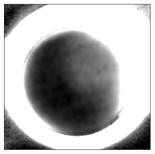
Image: Charon-lit-Pluto: The image shows the dark side of Pluto surrounded by a bright ring of sunlight scattered by haze in its atmosphere. But for a dark crescent zone to the left, the terrain is faintly illuminated by sunlight reflected by Pluto’s moon Charon. Researchers on the New Horizons team were able to generate this image using 360 images that New Horizons captured as it looked back on Pluto’s southern hemisphere. A large portion of the southern hemisphere was in seasonal darkness similar to winters in the Arctic and Antarctica on Earth, and was otherwise not visible to New Horizons during its 2015 flyby encounter of Pluto.
Credit: NASA/Johns Hopkins APL/Southwest Research Institute/NOIRLab.

This is Pluto’s southern hemisphere during the long transition into winter darkness; bear in mind that a winter on the distant world lasts 62 years. The all too faint light reflecting off Charon’s icy surface allows researchers to extract information. Tod Lauer (National Optical Infrared Astronomy Research Observatory, Tucson), lead author of a paper on the dark side work, compares available light here to moonlight on Earth:

“In a startling coincidence, the amount of light from Charon on Pluto is close to that of the Moon on Earth, at the same phase for each. At the time, the illumination of Charon on Pluto was similar to that from our own Moon on Earth when in its first-quarter phase.”

That’s precious little to work with, but the New Horizons Long Range Reconnaissance Imager (LORRI) made the best of it despite the fierce background light and the bright ring of atmospheric haze. We’ll have to wait a long time before the southern hemisphere is in sunlight, but for now, Pluto’s south pole seems to be covered in material darker than the paler surface of the northern hemisphere, with a brighter region midway between the south pole and the equator. In that zone we may have a nitrogen or methane ice deposit similar to the Tombaugh Regio ‘heart’ that is so prominent in the flyby images from New Horizons.

For more, see Lauer et al., “The Dark Side of Pluto,” Planetary Science Journal Vol. 2, No. 5 (20 Ocober 2021), 214 (abstract).

Of course, there is another mission that will forever have a holiday connection, at least if its planned liftoff on Christmas Eve happens on schedule. Dramatic days ahead.

All Your Base Are Belong To Us! : Alien Computer Programs

If you were crafting a transmission to another civilization — and we recently discussed Alexander Zaitsev’s multiple messages of this kind — how would you put it together? I’m not speaking of what you might want to tell ETI about humanity, but rather how you could make the message decipherable. In the second of three essays on SETI subjects, Brian McConnell now looks at enclosing computer algorithms within the message, and the implications for comprehension. What kind of information could algorithms contain vs. static messages? Could a transmission contain programs sufficiently complex as to create a form of consciousness if activated by the receiver’s technnologies? Brian is a communication systems engineer and expert in translation technology. His book The Alien Communication Handbook (Springer, 2021) is now available via Amazon, Springer and other booksellers.

by Brian S McConnell

In most depictions of SETI detection scenarios, the alien transmission is a static message, like the images on the Voyager Golden Record. But what if the message itself is composed of computer programs? What modes of communication might be possible? Why might an ETI prefer to include programs and how could they do so?

As we discussed in Communicating With Aliens : Observables Versus Qualia, an interstellar communication link is essentially an extreme version of a wireless network, one with the following characteristics:

Extreme latency due to the speed of light (eight years for round trip communication with the nearest solar system), and in the case of an inscribed matter probe, there may be no way to contact the sender (infinite latency).Prolonged disruptions to line of sight communication (due to the source not always being in view of SETI facilities as the Earth rotates).Duty cycle mismatch (it is extremely unlikely that the recipient will detect the transmission at its start and read it entirely in one pass).

Because of these factors, communication will work much better if the transmission is segmented so that parcels received out of order can be reassembled by the receiver, and so that those segments are encoded to enable the recipient to detect and correct errors without having to contact the transmitter and wait years for a response. This is known as forward error correction and is used throughout computing (to catch and fix disc read errors) and communication (to correct corrupted data from a noisy circuit).

While there are simple error correction methods, such as the N Modular Redundancy or majority vote code, these are not very robust and dramatically reduce the link’s information carrying capacity. There exist very robust error correction methods, such as the Reed Solomon coding used for storage media and space communication. These methods can correct for prolonged errors and dropouts, and the error correction codes can be tuned to compensate for an arbitrary amount of data loss.

In addition to being unreliable, the communication link’s information carrying capacity will likely be limited compared to the amount of information the transmitter may wish to send. Because of this, it will be desirable to compress data, using lossless compression algorithms, and possibly lossy compression algorithms (similar to the way JPEG and MPEG encoders work). Astute readers will notice a built-in conflict here. Data that is compressed and encoded for error correction will look like a series of random numbers to the receiver. Without knowledge about how the encoding and compression algorithms work, something that would be near impossible to guess, the receiver will be unable to recover the original unencoded data.

The iconic Blue Marble photo taken by the Apollo 17 astronauts. Credit: NASA.

The value of image compression can be clearly shown by comparing the file size for this image in several different encodings. The source image is 3000×3002 pixels. The raw uncompressed image, with three color channels with 8 bits per pixel per color channel, is 27 megabytes (216 megabits). If we apply a lossless compression algorithm, such as the PNG encoding, this is reduced to 12.9 megabytes (103 megabits), a 2.1:1 reduction. Applying a lossy compression algorithm, this is further reduced to 1.1 megabytes (8.8 megabits) for JPEG with quality set to 80, and 0.408 megabytes (3.2 megabits) for JPEG with quality set to 25, which results in a 66:1 Reduction.

Lossy compression algorithms enable impressive reductions in the amount of information needed to reconstruct an image, audio signal, or motion picture sequence, at the cost of some loss of information. If the sender is willing to tolerate some loss of detail, lossy compression will enable them to pack well over an order of magnitude more content into the same data channel. This isn’t to say they will use the same compression algorithms we do, although the underlying principles may be similar. They can also interleave compressed images, which will look like random noise to a naive viewer, with occasional uncompressed images, which will stand out, as we showed in Communicating with Aliens : Observables Versus Qualia.

So why not send programs that implement error correction and decompression algorithms? How could the sender teach us to recognize an alien programming language to implement them?

A programming language requires a small set of math and logic symbols, and is essentially a special case of a mathematical language. Let’s look at what we would need to define an interpreted language, call it ET BASIC if you like. An interpreted language is abstract, and is not tied to a specific type of hardware. Many of the most popular languages in use today, such as Python, are interpreted languages.

We’ll need the following symbols:

Delimiter symbols (something akin to open and close parentheses, to allow for the creation of nested or n-dimensional data structures)Basic math operations (addition, subtraction, multiplication, division, modulo/remainder)Comparison operations (is equal, is not equal, is greater than, is less than)Branching operations (if condition A is true, do this, otherwise do that)Read/write operations (to read or write data to/from virtual memory, aka variables, which can also be used to create input/output interfaces for the user to interact with)A mechanism to define reusable functions

Each of these symbols can be taught using a “solve for x” pattern within a plaintext primer that can be interleaved with other parts of the transmission. Let’s look at an example.

1 ? 1 = 2
1 ? 2 = 3
2 ? 1 = 3
2 ? 2 = 4
1 ? 3 = 4
3 ? 1 = 4
4 ? 0 = 4
0 ? 4 = 4

We can see right away that the unknown symbol refers to addition. Similar patterns can be used to define symbols for the rest of the basic operations needed to create an extensible language.

The last of the building blocks, a mechanism to define reusable functions, is especially useful. The sine function, for example, is used in a wide variety of calculations, and can be approximated via basic math operations using the Taylor series shown below:

And in expanded form as:

This can be written in Python as:

The sine() function we just defined can later be reused without repeating the lower level instructions used to calculate the sine of an angle. Notice that the series of calculations used reduce down to basic math and branching operations. In fact any program you use, whether it is a simple tic-tac-toe game or a complex simulation, reduces down to a small lexicon of fundamental operations. This is one of the most useful aspects of computer programs. Once you know the basic operations, you can build an interpreter that can run programs that are arbitrarily complex, just as you can run a JPEG viewer without knowing a thing about how lossy image compression works.

In the same way, the transmitter could define an “unpack” function that accepts a block of encoded data from the transmission as input, and produces error corrected, decompressed data as output. This is similar to what low level functions do to read data off a storage device.

Lossless compression will significantly increase the information carrying capacity of the channel, and also allow for raw, unencoded data to be very verbose and repetitive to facilitate compression. Lossy compression algorithms can be applied to some media types to achieve order of magnitude improvements, with the caveat that some information is lost during encoding. Meanwhile, deinterleaving and forward error correction algorithms can ensure that most information is received intact, or at least that damaged segments can be detected and flagged. The technical and economic arguments for including programs in a transmission are so strong, it would be surprising if at least part of a transmission were not algorithmic in nature.

There are many ways a programming language can be defined. I chose to use a Python based example as it is easy for us to read. Perhaps the sender will be similarly inclined to define the language at a higher level like this, and will assume the receiver can work out how to implement each operation in their hardware. On the other hand, they might describe a computing system at a lower level, for example by defining operations in terms of logic gates, which would enable them to precisely define how basic operations will be carried out.

Besides their practical utility in building a reliable communication link, programs open up whole other realms of communication with the receiver. Most importantly, they can interact with the user in real-time, thereby mooting the issue of delays due to the speed of light. Even compact and relatively simple programs can explain a lot.

Let’s imagine that ET wants to describe the dynamics of their solar system. An easy way to do this is with a numerical simulation. This type of program simulates the gravitational interactionsof N number of objects by summing up gravitational forces acting on each object and steps forward an increment of time to forecast where they will be, and then repeats this process ad infinitum. The program itself might only be a few kilobytes or tens of kilobytes in length since it just repeats a simple set of calculations many times. Additional information is required to initialize the simulation, probably on the order of about 50 bytes or 400 bits per object, enough to encode position and velocity in three dimensions at 64 bit accuracy. Simulating the orbits of the 1,000 most significant objects in the solar system would require less than 100 kilobytes for the program and its starting conditions. Not bad.

This is just scratching the surface of what can be done with programs. Their degree of sophistication is really only limited by the creativity of the sender, who we can probably assume has a lot more experience with computing than we do. We are just now exploring new approaches to machine learning, and have already succeeded at creating narrow AIs that exceed human capabilities in specialized tasks. We don’t know yet if generally intelligent systems are possible to build, but an advanced civilization that has had eons to explore this might have hit on ways to build AIs that are better and more computationally efficient than our state of the art. If that’s the case, it’s possible the transmission itself may be a form of Intelligence.

How would we go about parsing this type of information, and who would be involved? Unlike the signal detection effort, which is the province of a small number of astronomers and subject experts, the process of analyzing and comprehending the contents of the transmission will be open to anyone with an Internet connection and a hypothesis to test. One of the interesting things about programming languages is that many of the most popular languages were created by sole contributors, like Guido van Rossum, the creator of Python, or by small teams working within larger companies. The implication being that the most important contributions may come from people and small teams who are not involved in SETI at all.

For an example of a fully worked out system, Paul Fitzpatrick, then with the MIT CSAIL lab, created Cosmic OS, which details the ideas explored in this article and more. With Cosmic OS, he builds a Turing complete programming language that is based on just four basic symbols: 0 and 1, plus the equivalent of open and close parentheses.

There are risks and ethical considerations to ponder as well. In terms of risk, we may be able to run programs but not understand their inner workings or purpose. Already this is a problem with narrow AIs we have built. They learn from sets of examples instead of scripted instructions. Because of this they behave like black boxes. This poses a problem because an outside observer has no way of predicting how the AI will respond to different scenarios (one reason I don’t trust the autopilot on my Tesla car). In the case of a generally intelligent AI of extraterrestrial provenance, it goes without saying that we should be cautious in where we allow it to run.

There are ethical considerations as well. Suppose the transmission includes generally intelligent programs? Should they be considered a form of artificial life or consciousness? How would we know for sure? Should terminating their operation be considered the equivalent of murder, or something else? This idea may seem far fetched, but it is worthwhile to think about issues like this before a detection event.

Into the Atmosphere of a Star

We’ve been learning about the solar wind ever since the first interplanetary probes began to leave our planet’s magnetosphere to encounter this rapidly fluctuating stream of plasma. Finding a way to harness the flow could open fast transport to the outer Solar System if we can cope with the solar wind’s variability – no small matter – but in any case learning as much as possible about its mechanisms furthers our investigation of possible propulsive techniques. On this score and for the sake of solar science, we have much reason to thank the Parker Solar Probe and its band of controllers as the spacecraft continues to tighten its approaches to the Sun.

The spacecraft’s repeated passes by the Sun, each closer than the last, take advantage of speed and a heat shield to survive each perihelion event, and the last for which we have data was noteworthy indeed. During it, the Parker Solar Probe moved three separate times into and out of the Sun’s corona. This is a region where magnetic fields dominate the movement of particles. The Alfvén critical surface, which the spacecraft repeatedly crossed, is the boundary where the solar atmosphere effectively ends and the solar wind begins. Solar material surging up from below reaches a zone where gravity and magnetic fields can no longer hold it back. Breaking free, the solar wind effectively breaks the connection with the solar corona once across the Alfvén boundary.

So, as with our Voyagers moving past the heliopause and into interstellar space, we’ve accomplished another boundary crossing of consequence. A crossing into and back out of the corona helps define the location of the Alfvén critical surface, which turns out to be close to earlier estimates. These targeted a range between 10 and 20 solar radii. In its most recent passes by the Sun, the Parker Solar Probe has been below 20 solar radii, and on April 28 of this year, at 18.8 solar radii, it penetrated the Alfvén surface.

Nour Raouafi is a Parker project scientist at the Johns Hopkins Applied Physics Laboratory (JHU/APL):

“Flying so close to the Sun, Parker Solar Probe now senses conditions in the magnetically dominated layer of the solar atmosphere – the corona – that we never could before. We see evidence of being in the corona in magnetic field data, solar wind data, and visually in images. We can actually see the spacecraft flying through coronal structures that can be observed during a total solar eclipse.”

Image: As Parker Solar Probe passed through the corona on encounter nine, the spacecraft flew by structures called coronal streamers. These structures can be seen as bright features moving upward in the upper images and angled downward in the lower row. Such a view is only possible because the spacecraft flew above and below the streamers inside the corona. Until now, streamers have only been seen from afar. They are visible from Earth during total solar eclipses. Credit: NASA/Johns Hopkins APL/Naval Research Laboratory.

It’s clear from Parker data that the Alfvén surface is anything but smooth, and the spacecraft’s crossing into the corona did not in fact occur at perihelion on this particular pass, an indication of the varied structures within the region. As seen above, streamers and so-called pseudostreamers are found here, large magnetic-field structures streaming out of regions of the same magnetic polarity that are separated by an inner zone of opposite polarity. Caltech’s Christina M. S. Cohen explains the situation this way in a useful overview of the coronal crossing that notes the spacecraft’s fleeting passage through the boundary:

The center of a pseudostreamer is a region of enhanced magnetic field and reduced plasma density. This combination can push the Alfvén surface higher up in the corona, explaining why PSP’s orbit was able to cut across it…The period of time PSP spent below the Alfvén surface was too short to fully characterize the boundary and explore the inner region. Researchers expect that such a full characterization will require multiple expeditions carried out over different magnetic configurations and solar conditions.

It’s interesting to learn that we’re behind in acquiring data from the Parker Solar Probe because its high-gain antenna cannot be pointed toward Earth until it is far enough from the Sun on its current close pass to protect the equipment. Thus while the current data are from April of 2021, there was a likely crossing of the Alfvén critical surface again in November, when the probe reached a perihelion of 13.6 solar radii. This is close enough to suggest a longer period within the corona, something we won’t know until data download of that pass in late December.

Image: The solar corona during a total solar eclipse on Monday, August 21, 2017, above Madras, Oregon. The red light is emitted by charged iron particles at 1 million degrees Celsius and the green are those at 2 million degrees Celsius. On April 28, 2021, NASA’s Parker Solar Probe crossed the so-called Alfvén surface, entering, for the first time, a part of the solar corona that is “magnetically dominated.” Credit: M. Druckmuller / Christina M. S. Cohen.

Just as the Alfvén critical surface is anything but smooth, so too is the solar wind full of structure as it moves into the realm of the planets. So-called switchbacks were first detected by the Ulysses probe in the 1990s, what NASA describes as “bizarre S-shaped kinks in the solar wind’s magnetic field lines” which deflect charged particle paths as they move away from the Sun. The Parker Solar Probe discovered just how common these switchbacks were back in 2019, with later data showing that at least some switchbacks originate in the photosphere.

Switchbacks also align with magnetic funnels that emerge out of the photosphere between the convection cell structures called supergranules. It may be, then, that we can trace the origins of the solar wind at least partially to these magnetic funnels, as Stuart Bale (University of California, Berkeley) suggests:

“The structure of the regions with switchbacks matches up with a small magnetic funnel structure at the base of the corona. This is what we expect from some theories, and this pinpoints a source for the solar wind itself. My instinct is, as we go deeper into the mission and lower and closer to the Sun, we’re going to learn more about how magnetic funnels are connected to the switchbacks.”

Whether switchbacks are produced by the process of magnetic reconnection at the boundaries of magnetic funnels, or are produced by moving waves of plasma, is a question scientists hope the Parker Solar Probe will be able to answer. Just how the solar wind connects to switchbacks may help to explain how the corona is heated to temperatures far above that of the solar surface below. Bear in mind that the corona itself will be expanding as the Sun goes through its normal eleven year activity cycle, so we’ll have more opportunities for the Probe to pass through it.

Parker will eventually reach 8.86 solar radii, a scant 6.2 million kilometers from the solar surface, so this is a story that is far from over. The next flyby will be in January of 2022.

Findings from the recent Parker Solar Probe milestone will be published in The Astrophysical Journal, and are also examined in a paper by Kasper et al., “Parker Solar Probe Enters the Magnetically Dominated Solar Corona,” Physical Review Letters 127 (14 December 2021), 255101 (abstract).

Is Surface Ice Uncommon on Habitable Worlds?

The day is not far off when we’ll be able to look at a small planet in the habitable zone of its star and detect basic features on its surface: water, ice, land. The era of the 30-meter extremely large telescope approaches, so this may even be possible from the ground, and large space telescopes will be up to the challenge as well (which is why things like aperture size and starshade prospects loom large in our discussions of current policy decisions).

Consider this: On the Earth, while the atmosphere reflects a huge amount of light from the Sun, about half the total albedo at the poles comes from polar ice. It would be useful, then, to know more about the ice and land distribution that we might find on planets around other stars. This is the purpose of a new paper in the Planetary Science Journal recounting the creation of climate simulations designed to predict how surface ice will be distributed on Earth-like exoplanets. It’s a relatively simple model, the authors acknowledge, but one that allows rapid calculation of climate on a wide population of hypothetical planets.

Image: A composite of the ice cap covering Earth’s Arctic region — including the North Pole — taken 512 miles above our planet on April 12, 2018 by the NOAA-20 polar-orbiting satellite. Credit: NOAA.

Lead author Caitlyn Wilhelm (University of Washington) began the work while an undergraduate; she is now a research scientist at the university’s Virtual Planet Laboratory:

“Looking at ice coverage on an Earth-like planet can tell you a lot about whether it’s habitable. We wanted to understand all the parameters—the shape of the orbit, the axial tilt, the type of star—that affect whether you have ice on the surface, and if so, where.”

Thus we attempt to cancel out imprecision in the energy balance model (EBM) the paper deploys by sheer numbers, looking for general patterns like the fraction of planets with ice coverage and the location of their icy regions. A ‘baseline of expectations’ emerges for planets modeled to be like the Earth (which in this case means a modern Earth), worlds of similar mass, rotation, and atmospherics. The authors simulate more than 200,000 such worlds in habitable zone orbits.

What is being modeled here is the flow of energy between equator and pole as it sets off climate possibilities for the chosen population of simulated worlds over a one million year timespan. These are planets modeled to be in orbit around stars in the F-, G- and K-classes, which takes in our G-class Sun, and all of them are placed in the habitable zone of the host star. The simulations take in circular as well as eccentric orbits, and adjust axial tilt from 0 all the way to 90 degrees. By way of contrast, Earth’s axial tilt is 23.5 degrees. That of Uranus is close to 90 degrees. The choice of axial tilt obviously drives extreme variations in climate.

But let’s pause for a moment on that figure I just gave: 23.5 degrees. Because factors like this are not fixed, and Earth’s obliquity, the tilt of its spin axis, actually isn’t static. It ranges between roughly 22 degrees and 24.5 degrees over a timescale of some 20,000 years. Nor is the eccentricity of Earth’s orbit fixed at its current value. Over a longer time period, it ranges between a perfectly circular orbit (eccentricity = zero) to an eccentricity of 6 percent. While these changes seem small enough, they have serious consequences, such as the ice ages.

Image: The three main variations in Earth’s orbit linked to Milankovitch cycles. The eccentricity is the shape of Earth’s orbit; it oscillates over 100,000 years (or 100 k.y.). The obliquity is the tilt of Earth’s spin axis, and the precession is the alignment of the spin axis. Credit: Scott Rutherford. A good entry into all this is Sean Raymond’s blog planetplanet, where he offers an exploration of life-bearing worlds and the factors that influence habitability. An astrophysicist based in Bordeaux, Raymond’s name will be a familiar one to Centauri Dreams readers. I should add that he is not involved in the paper under discussion today.

Earth’s variations in orbit and axial tilt are referred to as Milankovitch cycles, after Serbian astronomer Milutin Milanković, who examined these factors in light of changing climatic conditions over long timescales back in the 1920s. These cycles can clearly bring about major variations in surface ice as their effects play out. If this is true of Earth, we would expect a wide range of climates on planets modeled this way, everything from hot, moist conditions to planet-spanning ‘snowball’ scenarios of the sort Earth once experienced.

So it’s striking that even with all the variation in orbit and axial tilt and the wide range in outcomes, only about 10 percent of the planets in this study produced even partial ice coverage. Rory Barnes (University of Washington) is a co-author of the paper:

“We essentially simulated Earth’s climate on worlds around different types of stars, and we find that in 90% of cases with liquid water on the surface, there are no ice sheets, like polar caps. When ice is present, we see that ice belts—permanent ice along the equator—are actually more likely than ice caps.”

Image. This is Figure 12 from the paper. Caption: Figure 12. Range and average ice heights of ice caps as a function of latitude for stars orbiting F (top), G (middle) and K (bottom) dwarf stars. Note the different scales of the x-axes. Light grey curves show 100 randomly selected individual simulations, while black shows the average of all simulations that concluded with an ice belt. Although the averages are all symmetric about the poles, some individual ice caps are significantly displaced. Credit: Wilhelm et al.

Breaking this down, the authors show that in their simulations, planets like Earth are most likely to be ice-free. Even oscillations in orbital eccentricity and axial tilt do not prevent, however, planets orbiting the F-, G- and K-class stars in the study from developing stable ice belts on land. Moreover, ice belts turn out to be twice as common as polar ice caps for planets around G- and K-class stars. As to size, the typical extension of an ice belt is between 10 and 30 degrees, varying with host star spectral type, and this is a signal large enough to show up in photometry and spectroscopy, making it a useful observable for future instruments.

This is a study that makes a number of assumptions in the name of taking a first cut at the ice coverage question, each of them “…made in the name of tractability as current computational software and hardware limitations prevent the broad parameter sweeps presented here to include these physics and still be completed in a reasonable amount of wallclock time. Future research that addresses these deficiencies could modify the results presented above.”

Fair enough. Among the factors that will need to be examined in continued research, all of them spelled out here, are geochemical processes like the carbonate-silicate cycle, ocean heat transport as it affects the stability of ice belts, zonal winds and cloud variability, all of this not embedded in the authors’ energy balance model, which is idealized and cannot encompass the entire range of effects. Nor do the authors simulate the frequency and location of M-dwarf planet ice sheets.

But the finding about the lack of ice in so many of the simulated planets remains a striking result. Let me quote the paper’s summation of the findings. They remove the planets ending in a moist greenhouse or snowball planet, these worlds being “by definition, uninhabitable.” We’re left with this:

…we then have 39,858 habitable F dwarf planets, 37,604 habitable G dwarf planets, and 36,921 habitable K dwarf planets in our sample. For G dwarf planets, the ice state frequencies are 92% ice free, 2.7% polar cap(s), and 4.8% ice belt. For F dwarf planets, the percentages are 96.1%, 2.9%, and 0.9%, respectively. For K dwarf planets, the percentages are 88.4%, 3.5%, and 7.6%, respectively. Thus, we predict the vast majority of habitable Earth-like planets of FGK stars will be ice free, that ice belts will be twice as common as caps for G and K dwarfs planets, and that ice caps will be three times as common as belts for Earth-like planets of F dwarfs.

And note that bit about the uninhabitability of snowball worlds, which the paper actually circles back to:

Our dynamic cases highlight the importance of considering currently ice-covered planets as potentially habitable because they may have recently possessed open surface water. Such worlds could still develop life in a manner similar to Earth, e.g. in wet/dry cycles on land, but then the dynamics of the planetary system force the planet into a snowball, which in turn forces life into the ocean under a solid ice surface. Such a process may have transpired multiple times on Earth, so we should expect similar processes to function on exoplanets.

The paper is Wilhelm et al., ”The Ice Coverage of Earth-like Planets Orbiting FGK Stars,” accepted at the Planetary Science Journal (preprint). Source code available. Scripts to generate data and figures also available.

Communicating With Aliens: Observables Versus Qualia

If we ever do receive a targeted message from another star – as opposed to picking up, say, leakage radiation – will we be able to decipher it? We can’t know in advance, but it’s a reasonable assumption that any civilization wanting to communicate will have strategies in place to ease the process. In today’s essay, Brian McConnell begins a discussion on SETI and interstellar messaging that will continue in coming weeks. The limits of our understanding are emphasized by the problem of qualia; in other words, how do different species express inner experience? But we begin with studies of other Earth species before moving on to data types and possible observables. A communication systems engineer and expert in translation technology, Brian is the author of The Alien Communication Handbook — So We Received A Signal, Now What?, recently published by Springer Nature under their Astronomer’s Bookshelf imprint, and available through Amazon, Springer and other booksellers.

by Brian McConnell

Animal Communication

What do our attempts to understand animal communication have to say about our future efforts to understand an alien transmission or information-bearing artifact, should we discover one? We have long sought to communicate with “aliens” here on Earth. The process of deciphering animal communication has many similarities with the process of analyzing and comprehending an ET transmission, as well as important differences. Let’s look at the example of audio communication among animals, as this is analogous to a modulated electromagnetic transmission.

The general methodology used is to record as many samples of communication and behavior as possible. This is one of the chief difficulties in animal communication research, as the process of collecting recordings is quite labor intensive, and in the case of animals that roam over large territories it may be impossible to observe them in much of their environment. Animals that have a small territory where they can be observed continuously are ideal.

Once these observations are collected, the next step is to understand the basic elements of communication, similar to phonemes in human speech or the letters in an alphabet. This is a challenging process as many animals communicate using sounds outside the range of human hearing, and employ sounds that are very different from human speech. This typically involves studying time versus frequency plots of audio recordings, to understand the structure of different utterances, which is also very labor intensive. This is one area where AI or deep learning can help greatly, as AI systems can be designed to automate this step, though they require a large sample corpus to be effective.

Time vs frequency plot of duck calls (click to enlarge).Credit: Brian McConnell.

The next step, once the basic units of communication are known, is to use statistical methods to understand how frequently they are used in conjunction with each other, and how they are grouped together. Zipf’s Law is an example of one method that can be used to understand the sophistication of a communication system. In human communication, we observe that the probability of a word being used is inversely proportional to its overall rank.

A log-log plot of the frequency of word use (y axis) versus word rank (x axis) from the text of Mary Shelley’s Frankenstein. Notice that the relationship is almost exactly 1/x. Image credit: Brian McConnell, The Alien Communication Handbook.

Conditional probability is another target for study. This refers to the probability that a particular symbol or utterance will follow another. In English, for example, letters are not used with equal frequency, and some pairs or triplets of letters are encountered much more often than others. Even without knowing what an utterance or group of utterances means, it is possible to understand which are used most often, and are likely most important. It is also possible to quantify the sophistication of the communication system using methods like this.

A graph of the relative frequency of use of bigrams (2 letter combinations) in English text (click to enlarge). You can see right away that some bigrams are used extensively while others very rarely occur.. Credit: Peter Norvig.

With this information in hand, it is now possible to start mapping utterances or groups of utterances to meanings. The best example of this to date is Con Slobodchikoff ’s work with prairie dogs. They turned out to be an ideal subject of study as they live in colonies, known as towns, and as such could be observed for extended periods of time in controlled experiments. Con and his team observed how their calls differed as various predators approached the town, and used a solve for x pattern to work out which utterances had unique meanings.

Using this approach, in combination with audio analysis, Con and his team worked out that prairie dogs had unique “words” for humans, coyotes and dogs, as well as modifiers (adjectives) such as short, tall, fat, thin, square shaped, oval shaped and carrying a gun. They did this by monitoring how their chirps varied as different predators approached, or as team members walked through with different color shirts, etc. They also found that the vocabulary of calls varied in different towns, which suggested that the communication was not purely instinctual but had learned components (cultural transmission). While nobody would argue that prairie dogs communicate at a human level, their communication does appear to pass many of the tests for language.

The challenge in understanding communication is that unless you can observe the communication and a direct response to something, it is very difficult to work out its meaning. One would presume that if prairie dogs communicate about predators, they communicate about other less obvious aspects of their environment that are more challenging to observe in controlled experiments. The problem is that this is akin to listening to a telephone conversation and trying to work out what is being said only by watching how one party responds.

Research with other species has been even more limited, mostly because of the twin difficulties of capturing a large corpus of recordings, along with direct observations of behavior. Marine mammals are a case in point. While statistical analysis of whale and dolphin communication suggests a high degree of sophistication, we have not yet succeeded in mapping their calls to specific meanings. This should improve with greater automation and AI based analysis. Indeed, Project CETI (Cetacean Translation Initiative) aims to use this approach to record a large corpus of whale codas and then apply machine learning techniques to better understand them.

That our success in understanding animal communication has been so limited may portend that we will have great difficulty in understanding an ET transmission, at least the parts that are akin to natural communication.

The success of our own communication relies upon the fact that we all have similar bodies and experiences around which we can build a shared vocabulary. We can’t assume that an intelligent alien species will have similar modes of perception or thought, and if they are AI based, they will be truly alien.

On the other hand, a species that is capable of designing interstellar communication links will also need to understand information theory and communication systems. An interstellar communication link is essentially an extreme case of a wireless network. If the transmission is intended for us, and they are attempting to communicate or share information, they will be able to design the transmission to facilitate comprehension. That intent is key. This is where the analogy to animal communication breaks down.

Observables

An important aspect of a well designed digital communication system is that it can interleave many different types of data or media types. Photographs are an example of one media type we may be likely to encounter. A civilization that is capable of interstellar communication will, by definition, be astronomically literate. Astronomy itself is heavily dependent on photography. This isn’t to say that vision will be their primary sense or mode of communication, just that in order to be successful at astronomy, they will need to understand photography. One can imagine a species whose primary sense is via echolocation, but has learned to translate images into a format they can understand, much as we have developed ultrasound technology to translate sound into images.

Digitized images are almost trivially easy to decode, as an image can be represented as an array of numbers. One need only guess the number of bits used per pixel, the least to most significant bit order, and one dimension of the array to successfully decode an image. If there are multiple color channels, there are a few additional parameters, but even then the parameter space is very small, and it will be possible to extract images if they are there. There are some additional encoding patterns to look for, such as bitplanes, which I discuss in more detail in the book, but even then the number of combinations to cycle through remains small.

The sender can help us out even further by including images of astronomical objects, such as planets, stars and distant nebulae. The latter are especially interesting because they can be observed by both parties, and can be used to guide the receiver in fine calibrations, such as the color channels used, scaling factors (e.g. gamma correction), etc. Meanwhile, images of planets are easy to spot, even in a raw bitstream, as they usually consist of a roundish object against a mostly black background.

An example of a raw bitstream that includes an image of a planet amid what appears to be random or efficiently encoded data. All the viewer needs to do to extract the image is to work out one dimension of the array along with the number of bits per pixel. The degree to which a circular object is stretched into an ellipse also hints at the number of bits per pixel. Credit: Brian McConnell, The Alien Communication Handbook.

What is particularly interesting about images is that once you have worked out the basic encoding schemes in use, you can decode any image that uses that encoding scheme. Images can represent scenes ranging from microscopic to cosmic scales. The sender could include images of anything, from important landmarks or sites to abstract representations of scenes (a.k.a. art). Astute readers will notice that these are uncompressed images, and that the sender may wish to employ various compression schemes to maximize the information carrying capacity of the communication channel. Compressed images will be much harder to recognize, but even if a relatively small fraction of images are uncompressed, they will stand out against what appears to be random digits, as in the example bitstream above.

Semantic Networks

The sender can take this a step further by linking observables (images, audio samples) with numeric symbols to create a semantic network. You can think of a semantic network like an Internet of ideas, where each unique idea has a numeric address. What’s more, the address space (the maximum number of ideas that can be represented) can be extremely large. For example, a 64 bit address space has almost 2 x 1019 unique addresses.

An example of a semantic network representing the relationship between different animals and their environment (click to enlarge). The network is shown in English for readability but the nodes and the operators that connect them could just as easily be based on a numeric address space.

The network doesn’t need to be especially sophisticated to enable the receiver to understand the relationships between symbols. In fact, the sender can employ a simple way of saying “This image contains the following things / symbols” by labeling them with one or more binary codes within the images themselves.

An example of an image that is labeled with four numeric codes representing properties within the image. Credit: Brian McConnell, The Alien Communication Handbook.

Observables Versus Qualia

While this pattern can be used to build up a large vocabulary of symbols that can be linked to observables (images, audio samples, and image sequences), it will be difficult to describe qualia (internal experiences). How would you describe the concept of sweetness to someone who can’t experience a sweet taste? You could try linking the concept to a diagram of a sugar molecule, but would the receiver make the connection between sugar and sweetness? Emotional states such as fear and hunger may be similarly difficult to convey. How would you describe the concept of ennui?

Imagine an alien species whose nervous system is more decentralized like an octopus. They might have a whole vocabulary around the concept of “brain lock”, where different sub brains can’t reach agreement on something. Where would we even start with understanding concepts like this? It’s likely that while we might be successful in understanding descriptions of physical objects and processes, and that’s not nothing, we may be flummoxed in understanding descriptions of internal experiences and thoughts. This is something we take for granted in human language, primarily because even with differences in language, we all share similar bodies and experiences around which we build our languages.

Yet all hope is not lost. Semantic networks allow a receiver to understand how unknown symbols are related to each other, even if they don’t understand their meaning directly. Let’s consider an example where the sender is defining a set of symbol codes we have no direct understanding of, but we have previously figured out the meaning of symbol codes that define set membership (∈), greater/lesser in degree (<>), and oppositeness (⋁) .

Even without knowing the meaning of these new symbol codes, the receiver can see how they are related and can build a graph of this network. This graph in turn can guide the receiver in learning unknown symbols. If a symbol is linked to many others in the network, there may be multiple paths toward working out its meaning in relation to symbols that have been learned previously. Even if these symbols remain unknown, the receiver has a way of knowing what they don’t know, and can map their progress in understanding.

The implication for a SETI detection is that we may find it is both easier and more difficult to understand what they are communicating than one may expect. Objects or processes that can be depicted numerically via images, audio or image sequences may enable the formation of a rich vocabulary around them and with relative ease, while communication around internal experiences, culture, etc may remain partially understood at best.

Even partial comprehension based on observables will be a significant achievement, as it will enable the communication of a wide range of subjects. And as can be shown, this can be done with static representations. An even more interesting scenario is if the transmission includes algorithms, functions from computer programs. Then it will be possible for the receiver to interact with them in real time, which enables a whole other realm of possibilities for communication.

More on that in the next article…