Aaron E. Carroll's Blog, page 3

Physician Tenure and Clinical Productivity

Health care systems nationwide face challenges in recruiting and retaining physicians, leading to high turnover and impact on patient care. Research also shows that new employees are often less productive than more experienced colleagues. If newly hired physicians take a long time to reach full productivity, the costs and effects of turnover on patient access may be greater than expected. Health systems may not be doing enough to ensure stable care during these transitions. Little research has examined how physician tenure affects productivity, leaving gaps in workforce planning and patient care strategies.

New Research

A recent retrospective cohort analysis published in the Journal of General Internal Medicine examined the relationship between physician tenure and clinical productivity in the Veterans Health Administration (VHA). The paper explored how tenure length affects productivity (i.e., the number of patient encounters per clinic day) among attending physicians. It also compared productivity trends between internally hired physicians—those who had any residency or fellowship training within the VHA—and externally hired physicians.

Methods

Researchers used the VHA’s Corporate Data Warehouse to collect detailed data on physician employment characteristics, specialty, and monthly patient encounters. Data was analyzed from 34,878 attending physicians across 27 specialties, covering over 1.5 million physician-months of outpatient encounters between October 1, 2017, and August 1, 2023. They used statistical models to examine productivity differences over time, adjusting for factors such as specialty, facility, and time effects, and sensitivity analyses to test the robustness of the results. The analyses were conducted for both the entire sample including all 27 specialties and four specialty subgroups—primary care, psychiatry, large medical specialties, and large surgical specialties.

Main Findings

Newly hired physicians had on average 1.72 fewer patient encounters per clinic day during their first quarter compared to their more experienced colleagues who had worked at VHA for more than two years. However, this productivity gap shrunk over time, with new hires having only 0.44 fewer encounters per clinic day by their eighth quarter. Among the specialty subgroups, medical and surgical specialty new hires reached productivity equivalent to more experienced employees by their eighth quarter. Additionally, physicians who had any residency or fellowship training within VHA (“internal hires”) had higher initial productivity and a quicker adjustment to full productivity than those hired externally, particularly in primary care and large surgical specialties.

Conclusion

These findings suggest that while newly hired attending physicians initially exhibit lower productivity, they experience significant improvement within the first two years. Moreover, those with prior VHA training adapt more quickly, highlighting the potential benefits of internal training programs. These insights are important for health care systems assessing the long-term costs and access implications associated with physician turnover and onboarding. Understanding these dynamics can aid in developing strategies to support new physicians, optimize training programs, and ultimately enhance patient care within VHA and similar health care settings.

The post Physician Tenure and Clinical Productivity first appeared on The Incidental Economist.

There’s a way to deal with brain injuries in football. It isn’t safety gear.

Tackle football and the National Football League (NFL) are heralded by most Americans as a staple of our country’s culture. It’s no wonder the Super Bowl breaks records for television viewership every year, for the game and the halftime show alike.  

Americans also know that football comes with head injuries, concussion, and even fatal illness like chronic traumatic encephalopathy (CTE). It’s a fact many of us have come to accept, sending our kids ourselves into play each season, knowing the risks.  

That has seemingly changed in recent years with the slow rise of protective equipment like the Guardian Cap and the Q-Collar. While uptake of this equipment is low so far, the NFL and others are praising its ability to protect athletes and make the game safer. The NFL also celebrated a decrease in concussions in 2024.  

But the bottom line is that no piece of equipment can prevent head injury in football. We should try to better respond to injury for both youth and professional athletes alike instead.  

TIE contributor Katherine O’Malley wrote about this in Harvard Public Health Magazine last week ahead of the big game.  

You can read the full piece here. 

The post There’s a way to deal with brain injuries in football. It isn’t safety gear. first appeared on The Incidental Economist.

Use of High-Risk Medications Among Older Adults Enrolled in Medicare Advantage Plans vs Traditional Medicare

When it comes time to visit a doctor, it’s common to have many priorities. Maybe it’s getting relief for that aggravated pickleball injury, taming a lingering cough or finally having that weird mole checked out [you really should]. Oftentimes the risks associated with our medications are not high on the priority list, but they should be.

While any medication has risks, understanding and managing those risks is more important for some prescription medications than others. High-risk (or high-alert) medications (HRMs) are those that present extreme danger either due to patient characteristics (e.g., age, chronic disease, etc.) or misuse. As such, HRMs require prescribers and health systems to employ a number of practices and tools to evaluate and mitigate risk towards improving patient safety.

Given their prevalence, there is mounting interest about prescribing practices of HRMs and the implications for health care.

Recent Study

In a study published in JAMA Network Open, evaluators from Harvard University and Boston University compared HRM prescribing trends between traditional fee-for-service Medicare (TM) and Medicare Advantage (MA), which are privately managed plans for Medicare eligible individuals that are publicly funded through a capitated payment arrangement.

To complete their analysis, the authors compared over 13.7 million matched pairs of beneficiaries taken from samples spanning 2013-2018. The study relied on several sources to obtain data on the sample population, including the Medicare Master Beneficiary Summary file, Social Vulnerability Index, U.S. Office of Management and Budget, and the Medicare Part D Master Beneficiary Summary File.

For its primary measure, the study relies on the Healthcare Effectiveness Data and Information Set (HEDIS) and its Use of High-Risk Medications in Older Adults (DAE) metric. As a primary outcome, the authors considered the total number of HRMs that were prescribed to the qualified enrollees. As a secondary outcome, the authors looked at the proportion of older enrollees who had been prescribed at least 1 HRM per year. Other outcomes included the proportion of enrollees who had received 2 or more HRMs per year or the same HRM twice in the same year.

In addition to the primary variable of Medicare insurance type (i.e., enrollment in TM vs. MA), the study also examined a number of covariates. The researchers considered age, sex, race and ethnicity, dual-eligibility status, rurality, social vulnerability, eligibility for Medicare’s low-income subsidy, and a patient health indicator that factors the number of non-HRM medications.

The authors first used linear regressions to construct their primary model, and after accounting for covariates and other effects (fixed and random), they plotted the adjusted rate of unique HRM prescriptions. After the secondary outcomes were plotted similarly, sensitivity analyses were completed according to a range of criteria.

Ultimately, the study found that the rate of HRM use decreased in each year of the study period (2013-2018) – this was true for both TM and MA alike. Consistent with previously observed prescribing trends, HRM use in MA was significantly lower than in TM, but the gap between the two had narrowed. In the final year of the study period, the rate of HRM use in TM was still 56.9 HRMs (per 1000 beneficiaries) compared to 41.5 in MA. Similar patterns were observed in the analyses of the secondary outcome of the proportion of enrollees who had been prescribed at least 1 HRM per year. When compared with TM, MA performed better with a lower adjusted proportion of beneficiaries who had been prescribed at least 1 HRM (3.9%) versus 5.3% in TM. Relative to patient characteristics, the study observed higher rates of HRM use for certain population subgroups, including those who were female, American Indian or Alaska Native, or White.

Conclusion

The authors note several key limitations, including limiting analyses to only those medications identified by the DAE measure during the study period. The study was also unable to assess the extent that the HRM prescribing were clinically appropriate. The authors also explain that this work is limited by the use of MA as a single exposure and that only filled prescriptions were included in the analyses.

Despite these limitations, this study has implications for both medical practice and health care policy. As the study found that certain populations (female, American Indian or Alaska Native, and White individuals) received HRMs with greater frequency, there is a need to better understand how prescribers assess clinical presentation of these populations. The study’s findings also highlight how the mechanisms responsible for the overall decrease in HRM use in TM are not entirely known. The authors recommend that the Centers for Medicare & Medicaid Services explore additional avenues (e.g., tying HRM rates to reimbursement models) to narrow the gap between TM and MA relative to HRM rates.

Given their potential for harm, further research into HRM medication management strategies is an essential component of improving patient care and safety for older adults.

The post Use of High-Risk Medications Among Older Adults Enrolled in Medicare Advantage Plans vs Traditional Medicare first appeared on The Incidental Economist.

Can We Engineer the Environment to Avoid Junk Foods?

Can we change our behavior by changing the environment? A lot of junk food is available in the checkout lanes at grocery stores. Most of us are susceptible to it, and just about everybody impulse buys a candy bar now and again. What happens when we control what’s available in checkouts? Does changing the environment change people’s behavior?

 



The post Can We Engineer the Environment to Avoid Junk Foods? first appeared on The Incidental Economist.

Coastal Living May Endanger Your Life

Coastal living is a dream for many Americans, but the growing impacts of climate change are making it increasingly risky. In my recent piece for The Portland Press Herald, I explore how climate change is affecting coastal areas and those residents’ health. I also shed light on the solutions already in progress.

Read the full article here.

The post Coastal Living May Endanger Your Life first appeared on The Incidental Economist.

Covid Vaccine Misinformation or Disinformation? Which Was Worse?

In May 2024 a set of articles were published in the journal Science that focused on the intersection of misinformation and social media. The results, while preliminary in the grand scheme of things, were really interesting (and maybe a little alarming).

 



The post Covid Vaccine Misinformation or Disinformation? Which Was Worse? first appeared on The Incidental Economist.

Trump’s Return Puts Inflation Reduction Act in Jeopardy

With the rise in prescription drug prices in recent years, many Americans have been forced to choose between paying for medication and other necessities like rent or groceries. The passage of the Inflation Reduction Act in 2022 changed that for those on Medicare, providing some relief by capping costs for beneficiaries.  

That progress is now in jeopardy with a new Trump administration that has voiced support for repeal of the Inflation Reduction Act’s protections. Doing so could also squash any hope for extending prescription drug price protections for a much larger portion of Americans: the privately insured.  

I wrote about that for Public Health Post. Read the full piece here.  

Research for this article was supported by Arnold Ventures.

The post Trump’s Return Puts Inflation Reduction Act in Jeopardy first appeared on The Incidental Economist.

A Bit More on Physical Pendulum Isochronal Pivot Points

This is a follow-up post to this one, which you should (re)read if this topic is of interest to you and any of the following is unfamiliar. The same warning about mobile viewing applies: all square roots are over both numerator and denominator, despite how it may appear on a mobile device.

A physical pendulum with mass m and center of mass (CM) moment of inertia Icm pivoting at a point d from the CM has period T given by

T=2πIcm+md2mgdT = 2\pi \sqrt{\frac{I_{\text{cm}} + md^2}{mgd}}

with g being the acceleration due to gravity. The last post showed that T has the same value on two circles centered on the pendulum’s CM, one with radius d and one with radius d’, where d’ = L – d and

L=Imd

Here I = Icm+ md2. The CM-centered circles of radius d and d’ are composed of isochronal points. That is, the period is the same no matter which point on these circles the pendulum is pivoted about.

This post explores T as a function of d (or d’) and some properties of d.

How T Behaves as d Varies

T as a function of d has a shape as shown in the figure below, where the horizontal and vertical axes represent d and T, respectively.

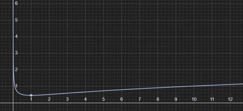
This suggests T approaches infinity as d approaches zero or infinity. This can be shown formally by taking limits, but it’s not hard to see informally by examining the expression for T.

As d approaches zero, the expression for T resembles (or behaves like) a constant times the inverse of the square root of d, which is asymptotic to the T-axis in the above plot and certainly goes to infinity. As d approaches infinity, the expression for T behaves like a constant times the square root of d, which also goes to infinity, as the graph shows.

This behavior of T as d approaches zero or infinity makes sense. As d approaches zero, the pendulum’s pivot point approaches its CM. There is no restoring torque at the CM, and the pendulum would not return from a displacement. Think of turning a disk of uniform density pinned at the center (its CM). If you give it a turn, it won’t turn back. That’s an infinite period.

As d approaches infinity, the situation resembles a simple pendulum, for which the period is proportional to the square root of its length (d), hence T also approaches infinity.

Moving away from these extremes, T strictly monotonically decreases to a minimum. This itself means that the minimum must be where d=d’. If this were not the case, then there would be two isochronal circles, centered on the CM, of minimum T, one of radius d and one of radius d’. This would imply that all pivot points a distance r from the CM such that dhave larger periods, which contradicts the strict monotonicity of T from zero (or infinity) to the minimum.

Or, we could take the derivative of T with respect to d and set it to zero (steps omitted) to find that the minimum T is where

d2=Icmmd^2 = \frac{I_{\text{cm}}}{m}

From the previous post, this is also the expression for dd’. That means that the minimum T is found where d and d’ coincide. This value of d is also the radius of gyration. By definition, this is the radius such that if all of m resided there, the moment of inertia would be the same as the object’s (here the pendulum) with distributed mass.

Plugging this into the expression for T given above, the minimum T (or, for convenience, T2) is

Tmin2=8π2gIcmm

So, when d=0, d’=∞ we have two (degenerate) isochronal circles for which T is infinite. As d moves radially outward from the CM, d’ moves inward, and the circles they define are always composed of isochronal points. As this happens, T drops from infinity toward a unique minimum proportional to the quartic root of Icm/m. The minimum is achieved when d=d’, at the radius of gyration, and the two isochronal circles become one (♥ cue violins ♥).

Where is the Minimum with Respect to the Pendulum?

Where is the d for which T is minimum with respect to the boundary of the pendulum? It’s never outside the boundary of the pendulum. I’ll show this mathematically, below, but it’s intuitive. Lengthening a simple pendulum, for which all the mass is at the end of the (assumed massless) support, increases its period. So, it stands to reason that a pivot point beyond the surface of a physical pendulum would have a larger period than a pivot point on its surface. Also, the definition of radius of gyration makes it pretty clear that it’s within the pendulum.

Let’s do it with math anyway. The pendulum’s CM rotational inertia is, by definition

Icm=∫r2 dmI_{\text{cm}} = \int r^2 \, dm

where r is the perpendicular distance from the CM to a infinitesimal mass element dm. Replacing r with rmax, the largest distance from the CM to the boundary of the pendulum, we get the inequality

Icm=∫r2 dm≤rmax2∫dmI_{\text{cm}} = \int r^2 \, dm \leq r_{\text{max}}^2 \int dm

Or, simply,

Icm≤rmax2 mI_{\text{cm}} \leq r_{\text{max}}^2 \, m

Substituting this into the expression for the T-minimizing d above, d ≤ rmax. Equality is obtained only when all the pendulum’s mass is at a constant radius from the CM (an idealized hoop of zero width). Otherwise, the T-minimizing d is strictly within the pendulum’s boundary. For all practical purposes (assuming there are any), d < rmax. That is, not only is the T-minimizing d not outside the pendulum, it’s not even on the surface (apart from the idealized hoop). It’s somewhere strictly inside the pendulum. That means that both d and d’ are within the boundary of the pendulum for some range.

If the body of the pendulum includes the CM (true for convex shapes like a disk or triangle), then all possible values of T, from its maximum of infinity to its minimum at the d defined above are found at pivot points within it. For all such values of T, there are arcs* of one or two isochronal circles within the body of the pendulum — one when d’ is outside the pendulum’s boundary and two when it is inside, which, as noted above, it will be for some range. In fact, that range is when d’ is between the T-minimizing d (the radius of gyration) and rmax. 

If the body of the pendulum does not include the CM (as would be the case for some concave shapes like a uniform density banana or a washer), the maximum T for which a pivot point is inside the body of the pendulum is given by

T=2πIcm+mrmin2mgrminT = 2\pi \sqrt{\frac{I_{\text{cm}} + m r_{\text{min}}^2}{m g r_{\text{min}}}}

where rmin is the distance from the CM to the point within the pendulum closest to it.​

Summary

The period of a physical pendulum, T, varies with pivot point from infinity (at pivot points CM and infinity) to a minimum at the radius of gyration.​A minimum achieving pivot point is always within the body of the pendulum. If the body of the pendulum includes the CM, then for all possible values of T, from its minimum to infinity, there are arcs of one or two isochronal circles within the body of the pendulum.​If the body of the pendulum does not include the CM, there are only isochronal circle arcs for T less then a finite maximum value, an expression for which we found.

* I’m talking arcs of circles and not necessarily full circles here because there may be some radial distances from the CM for which the body of the pendulum exists for only some angles. Think of a triangular-shaped pendulum as opposed to a disk-shape one. For the former, there are some CM-centered circles of radius less than the extent of the triangle that aren’t entirely within the triangle. For the latter, this is not true.

The post A Bit More on Physical Pendulum Isochronal Pivot Points first appeared on The Incidental Economist.

The Geometry of Isochronal Pivot Points for a Physical Pendulum

Note that if you’re reading this on a mobile device, some of the equations don’t look right. In particular, one thing I noticed is that the square root radical over a fraction appears to only be over the numerator. All such square roots are over the denominator too. The equations look right (to me) when viewed on a non-mobile device (e.g., my laptop).

This post is about a topic in physics, which I suspect may not be of interest to many regular TIE readers. But, it could interest irregular (?) readers.

Why physics? It was my undergrad major, and I’m now helping my daughter through AP Physics. I’m finding myself going down some rabbit holes, exploring things I didn’t learn in college. Some aren’t in any textbook I have at my fingertips or online (so far as I can tell). This post is about one such thing. I used AI to check the math and logic. If you see a problem, please let me know.

What This Post Shows
Our starting point is a well-known property of a physical pendulum (also called a compound pendulum), the discovery of which is credited to Christian Huygens: you can pivot the pendulum from two different points and get the same period (they’re isochronal). Given one pivot point, Huygens and any other basic physics text that covers this topic, shows how to find “the” other isochronal pivot point.

What this post shows is that, in fact, there are an infinite number of isochronal points (hence the quotes around “the” in the previous sentence). Moreover, they all lie on two circles about the center of mass (CM).

The First Isochronal Circle
The derivation for the period of a physical pendulum can be found online or in many textbooks. The period T about pivot point P is given by

T=2πImgdT = 2\pi \sqrt{\frac{I}{mgd}}

where I is the moment of inertia about the pivot point, m is the pendulum’s mass, g is the acceleration due to gravity, and d is the distance between P and the CM. From the parallel axis theorem

I=ICM+md2I = I_{\text{CM}} + m d^2

where the first term is the moment of inertia about the center of mass. Therefore,

T=2πICM+md2mgdT = 2\pi \sqrt{\frac{I_{\text{CM}} + m d^2}{m g d}}

which is constant for any distance d from the CM in any direction. Thus, there are infinite isochronal pivot points that lie on a circle of radius d centered on the CM. This is the first isochronal circle.​​

The Second Isochronal Circle
As discussed in many places but not shown in a simple way (that I’ve seen), there is a pivot point isochronal with P and not on the circle described above. It’s called the center of oscillation and we’ll label it point Q. The end of this post has a straightforward proof that the isochronal point Q is a distance L from P through the CM where

L=ImdL = \frac{I}{md}

Define d’ = L – d as the distance between Q and the CM. The physical pendulum has a moment of inertia I’ about point Q. We can plug d’ and I’ into the equations provided in the section above (The First Isochronal Circle). The conclusion follows by the same argument as above that the period is a constant T for any point a distance d’ from the CM. We know it is T (the same period as in the previous section) because P and Q are isochronal pivot points. Thus there are an infinite isochronal pivot points that lie on a circle of radius d’ centered on the CM. This is the second isochronal circle.

Or, to sum up, Huygens and countless others open our eyes to the fact that there are two isochronal points, P and Q. What is also true is that there are two isochronal circles about the CM, one contains P, the other Q.

This is consistent with the obvious fact that the period of oscillation of a uniform density rod pivoting at one end is the same as that pivoting on the other end (an isochronal circle goes through both ends). Or, the period of oscillation is the same for any point of a circular disk of uniform density equidistant from the center (isochronal circles are concentric about the CM). These obvious facts are clear to us from symmetry.

What’s given above shows that the circular isochronal symmetry is there even for asymmetric (arbitrarily shaped, with non-uniform density) physical pendulums. This is not intuitive (not to me anyway). Yet, the only thing that isn’t fixed for all points relating to a given pendulum in the expression for T is the distance of the pivot point from the CM. With that, isochronal circularity is unavoidable.

Conclusion
Notice that d can be any positive distance, giving rise to any positive period T. So, by the above arguments, all isochronal pivot points lie on pairs of concentric circles centered about the CM. (There is a small technicality that for some (OK, an infinite number of) values of d, some isochronal points may not be within the body of the pendulum. That doesn’t mean they’re not isochronal with the other points on the circle(s) associated with d (or d’). It just means that actually getting the pendulum to pivot around such a point is challenging in practice. It’d take a massless, unbending support from that point to the pendulum’s CM.)

Proof That the Center of Oscillation is Isochronal (Or Pivot Q Has the Same Period as Pivot P)
Above, I promised this proof. Skip it if you’re willing to trust Huygens and countless other physics texts, some of which state this without proof.

With all the terms as defined in the post, start with some preliminary stuff to get an expression of d’ in terms of d that will be useful later. Recall that

L=ImdL = \frac{I}{m d},

By the parallel axis theorem, and as noted in the post

I=ICM+md2

Therefore,

L=ICM+md2mdL = \frac{I_{\text{CM}} + m d^2}{m d}.

And, simplifying,

L=ICMmd+dL = \frac{I_{\text{CM}}}{m d} + d.

Using this and the definition of d’ (= L – d) from the post, we have

d′=(ICMmd+d)−dd’ = \left(\frac{I_{\text{CM}}}{m d} + d\right) – d.

So that

d′=ICMmdd’ = \frac{I_{\text{CM}}}{m d}.

The period of the pendulum pivoting about point Q is given by

T′=2πI′mgd′T’ = 2\pi \sqrt{\frac{I’}{m g d’}},

The job is to show T’=T. We will do so by plugging in for I’ and d’ and doing some algebra. Here we go. The only thing we can do with I’ is apply the parallel axis theorem.

I′=ICM+md′2.I’ = I_{\text{CM}} + m d’^2.

Plug in the expression for d’ from above. (This is why we did that preliminary work.)

I′=ICM+m(ICMmd)2 I’ = I_{\text{CM}} + m \left(\frac{I_{\text{CM}}}{m d}\right)^2.

Cancel m and plug this into the numerator of T’ and use the expression for d’ in the denominator too.

T′=2πICM+ICM2md2mg⋅ICMmd.T’ = 2\pi \sqrt{\frac{I_{\text{CM}} + \frac{I_{\text{CM}}^2}{m d^2}}{m g \cdot \frac{I_{\text{CM}}}{m d}}}.

There’s lots to cancel to simplify. Go ahead and do that on a scrap of paper or in your head. You’ll get

T′=2π1+ICMmd2gdT’ = 2\pi \sqrt{\frac{1 + \frac{I_{\text{CM}}}{m d^2}}{\frac{g}{d}}}.

Multiply numerator and denominator in the square root by md2 to get

2πICM+md2mgdT = 2\pi \sqrt{\frac{I}{m g d}} = 2\pi \sqrt{\frac{I_{\text{CM}} + m d^2}{m g d}}.

Recognize, from the parallel axis theorem, that the numerator is just I and that this is the expression for T. So, T’ = T and we are done.

The post The Geometry of Isochronal Pivot Points for a Physical Pendulum first appeared on The Incidental Economist.

Like the EpiPen, but cheaper, smaller, and no needle

There’s been a fair amount of good news on the allergy front lately, including a medication for food allergies that we covered recently, and now some good news for anyone compelled to carry around an EpiPen. A new alternative for people at risk of anaphylaxis is smaller, easier to use, and doesn’t even use a needle! Here’s what we know about Neffy.

 



The post Like the EpiPen, but cheaper, smaller, and no needle first appeared on The Incidental Economist.