Paul Gilster's Blog, page 100

Water Delivery to the Early Earth

Thinking about supplying a young planet with water, the mind naturally heads for the outer reaches of the Solar System. After all, beyond the ‘snowline,’ where temperatures are cold enough to allow water to condense into ice grains, volatiles are abundant (this also takes in methane, ammonia and carbon dioxide, all of which can condense into ice grains). The idea that comets or water-rich asteroids bumping around in a chaotic early Solar System could deliver the water Earth needed for its oceans makes sense, given our planet’s formation well inside the snowline.

We’ve just looked at Ceres, in celebration of the Dawn mission’s achievements there, and we know that Ceres has an icy mantle and perhaps even an ocean beneath its surface. At 2.7 AU, the dwarf planet is right on the edge of traditional estimates for the snowline as it would have occurred in the early days of planet formation. Obviously, the snowline has a great deal to do with various models about the accretion of solid grains into planetesimals.

If I dig around in the archives, I can even show you an image of a snowline. The star below is V883 Orionis, from a stellar class called FU Orionis, a young, pre-main sequence star capable of major variability in brightness and spectral type. The snowline is easy to find here because an outburst in luminosity has heated up the protoplanetary disk, pushing the snowline outwards.

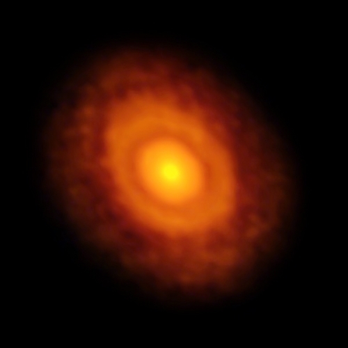
Image: This image of the planet-forming disc around the young star V883 Orionis was obtained by ALMA in long-baseline mode. This star is currently in outburst, which has pushed the water snowline further from the star and allowed it to be detected for the first time. The dark ring midway through the disc is the water snowline, the point from the star where the temperature and pressure dip low enough for water ice to form. Credit: ALMA (ESO/NAOJ/NRAO)/L. Cieza.

As sound an idea as water delivery via objects from beyond the snowline seems, it’s always wise to question our assumptions, and indeed, the issue is strongly debated. For a second scenario for Earth’s water is available. This is the idea that enough water-rich dust grains can accumulate to form boulders of kilometer size, objects that can contain large enough amounts of water to explain the amount we have on Earth. This is the so-called ‘wet-endogenous scenario,’ in which water in the early, still accreting Earth occurs in the form of hydrous silicates.

An interesting take on this comes from Martina D’Angelo (University of Groningen, the Netherlands) and colleagues, with a second paper in the process from W. F. Thi (Max Planck Institute for Extraterrestrial Physics) and team. How to defend the latter scenario given Earth’s formation well inside the snowline? The answer may lie in sheets of silicate materials called phyllosilicates, which as I’ve learned in preparing this piece, include the micas, chlorite, serpentine, talc, and the clay minerals. Usefully, they have interesting properties when it comes to water, retaining it when heated up to several hundreds of degrees centigrade.

Thus D’Angelo, supported by earlier work, notes that there is a way to preserve structural water even in the warmer regions of the protoplanetary disk. D’Angelo’s paper, supported by the still unpublished work of Thi’s team, explores how water from the gas phase can diffuse into the silicates well before the dust grains of the inner system have accreted into planetesimals.

The paper explains the astrophysical models for protoplanetary disks and the Monte Carlo simulations used for studying ice accretion on grains that were used in this work. The simulations show water vapor abundances, temperature and pressure radial profiles that identify where in the protoplanetary disk hydration of dust grains could have occurred. The results show that the ‘wet endogenous scenario’ can by no means be ruled out. From the paper, addressing the simulation results for water adsorption on a forsterite crystal lattice:

Our MC [Monte Carlo] models show that complete surface water coverage is reached for temperatures between 300 and 500 K. For hotter environments (600, 700 and 800 K), less than 30% of the surface is hydrated. At low water vapor density and high temperature, water cluster formation plays a crucial role in enhancing the coverage… The binding energy of adsorbed water molecules increases with the number of occupied neighboring sites, enabling a more temperature-stable water layer to form. Lateral diffusion of water molecules lowers the timescale for surface hydration by water vapor condensation by three order of magnitude with respect to an SCT model, ruling out any doubts on the efficiency of such process in a nebular setting.

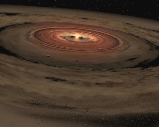
Image: Artist impression of a very young star surrounded by a disk of gas and dust. Scientists suspect that rocky planets such as the Earth are formed from these materials. Credit & Copyright: NASA/JPL-Caltech.

D’Angelo and colleagues believe that between 0.5 and 10 Earth oceans worth of water can be produced by the agglomeration of hydrated grains in an Earth-sized planet in formation, depending on size differences among the grains. The timescale in question fits easily into the time necessary for grains to eventually accrete into larger boulders within the early Solar nebula. Now needed are simulations of grain growth that will help the researchers understand how water is retained on grain surfaces through periods of accumulation and collision.

So it may be that we have twin processes at work, with delivery of water from comets and asteroids playing a role in bulking up a young world with a latent supply of its own water.

The papers are Thi et al., “Warm dust surface chemistry in protoplanetary disks – Formation of phyllosilicates,” submitted to Astronomy & Astrophysics, and D’Angelo et al., “On water delivery in the inner solar nebula: Monte Carlo simulations of forsterite hydration,” accepted at Astronomy & Astrophysics (preprint).

FRB 121102: New Bursts From Older Data

“Not all discoveries come from new observations,” says Pete Worden, in a comment referring to original thinking as applied to an existing dataset. Worden is executive director of the Breakthrough Initiatives program, which includes Breakthrough Listen, an ambitious attempt to use SETI techniques to search for signs of technological activity in the universe. Note that last word: The targets Breakthrough Listen examines do extend to about one million stars in the stellar neighborhood, but they also go well outside the Milky Way, with 100 galaxies being studied in a range of radio and optical bands.

A major and sometimes neglected aspect of SETI as it is reported in the media is the fact that such careful observation can turn up highly useful astronomical information unrelated to any extraterrestrial technologies. Worden’s comment underlines the fact that we are generating vast data archives as our multiplying space- and ground-based instruments continue to scan the heavens at various wavelengths. It is not inconceivable that the signature of a distant civilization or a novel astrophysical process is buried deep within data that is years or decades old.

The case in point this morning comes through Breakthrough Listen’s observations of the Fast Radio Burst (FRB) 121102. FRBs seize the attention because they are a recent and puzzling detection. The first, the so-called Lorimer Burst (FRB 010724) was found no more than eleven years ago. FRBs are also highly unusual, appearing as radio pulses of extremely short duration, usually milliseconds. They are believed to originate in distant galaxies and one of them, FRB 121102, stands out because unlike all others thus far detected, it sends out repeat bursts.

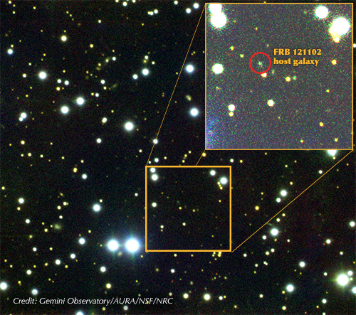
Image: The FRB in question. This is a Gemini composite image of the field around FRB 121102 (indicated). The dwarf host galaxy was imaged, and spectroscopy performed, using the Gemini Multi-Object Spectrograph (GMOS) on the Gemini North telescope on Maunakea in Hawai’i. Data were obtained on October 24-25 and November 2, 2016, before the subsequent Breakthrough Listen observations at Green Bank. Credit: Gemini Observatory/AURA/NSF/NRC.

FRB 121102 is prolific in repeat bursts, as it turns out, and this is where Worden’s words resonate. Earlier studies have shown that the source is located in a galaxy some 3 billion light years away. Breakthrough Listen’s observing team at the University of California, Berkeley SETI Research Center went to work on this ‘repeater’ on August 26, 2017, finding a total of 21 bursts in data acquired at the Green Bank Telescope in West Virginia. All of these turned up within a single hour, which implies periods of intense activity. For more, see New Activity of Repeating FRB 121102.

Working with the same dataset, UC Berkeley graduate student Gerry Zhang and collaborators have now introduced a new machine learning algorithm into the mix, subjecting the same dataset (about 400 TB) to techniques not dissimilar to those used by Internet technology companies. Zhang and team’s ‘convolutional neural network’ was trained to recognize FRBs in the same way that Vishal Gajjar applied when he and his own colleagues analyzed the data in 2017. The algorithm was then applied to the raw data to see if anything new could be acquired.

From the paper:

…we present a re-analysis of the C-band observation by Breakthrough Listen on August 26, 2017 with convolutional neural networks. Recent rapid development of deep learning, and in particular, convolutional neural networks (CNN; Krizhevsky et al. 2012; Simonyan & Zisserman 2014; He et al. 2015; Szegedy et al. 2014) has enabled revolutionary improvements to signal classification, pattern recognition in all fields of data science such as, but not limited to computer image processing, medicine, and autonomous driving. In this work, we present the first successful application of deep learning to direct detection of fast radio transient signals in raw spectrogram data.

The result: 72 new detections of pulses from FRB 121102. That takes the cumulative total from this dataset to 93 pulses in five hours of observation, including 45 pulses within the first 30 minutes. As to periodicity, the work shows that the pulses are not received in a regular pattern. Using the same methods, Zhang and team go on to explore trends in pulse fluence, pulse detection rate, and pulse frequency structure. The breadth of the analysis is made possible by the sheer number of pulses, the highest detected from a single observation, and the use of Zhang and team’s neural network technology, which can surely be adapted to other datasets.

“Gerry’s work is exciting not just because it helps us understand the dynamic behavior of FRBs in more detail,” says Berkeley SETI Research Center Director and Breakthrough Listen Principal Investigator Dr. Andrew Siemion, “but also because of the promise it shows for using machine learning to detect signals missed by classical algorithms.”

So can we be sure we are dealing with a natural astrophysical phenomenon, or is there any possibility of a technology behind this repeating FRB? The data here do not give us the answer, but it’s intriguing to speculate about galactic SETI in light of our recent discussion of the work of Yuki Nishino and Naoki Seto (Kyoto University), who have suggested that natural phenomena such as the merger of a binary neutron star system like GW170817 could be used as a marker to flag a message from a civilization attempting to announce its presence to the cosmos.

For that matter, are all FRBs the same? We’ve only found the one repeater thus far, but 104 are now thought to occur in our sky on a daily basis. Avi Loeb and Minasvi Lingam (Harvard University) have worked out an FRB rate for each galaxy within 100 Gpc3 of about 10-5 per day, if indeed we are dealing with natural sources like gamma ray bursts or neutron star mergers. And as they’ve noted in a recent paper, one of these going off in our own galaxy, as would be expected about every 300 years, would resolve the question of FRB origins, a doubtless spectacular event if occurring nearby.

The Gajjar et al. paper reporting on the 2017 repeat detections is “Highest-frequency detection of FRB 121102 at 4-8 GHz using the Breakthrough Listen Digital Backend at the Green Bank Telescope,” accepted at The Astrophysical Journal (preprint). The Zhang et al. paper covering the subsequent new analysis is “Fast Radio Burst 121102 Pulse Detection and Periodicity: A Machine Learning Approach,” accepted for publication in The Astrophysical Journal, with further details available here. Avi Loeb and Minasvi Lingam’s paper on technological possibilities in FRBs is “Fast Radio Bursts from Extragalactic Light Sails,” The Astrophysical Journal Letters Vol. 837, No. 2 (March 8, 2017). Abstract / preprint.

Dawn at Sunset

The announcement that the Dawn spacecraft is running out of its hydrazine fuel was not unexpected, but when we prepare to lose communications with a trailblazing craft, the moment is always tinged with a bit of melancholy. Even so, the accomplishments of this mission in its 11 years of data gathering are phenomenal. They also speak to the virtues of extended missions, which in this case gave us views and a wealth of information about Vesta but also a continuation of its stunning orbital operations around Ceres. And at Ceres it will stay, a silent orbiting monument to deep space exploration.

“Dawn’s legacy is that it explored two of the last uncharted worlds in the inner Solar System,” said Marc Rayman of NASA’s Jet Propulsion Laboratory in Pasadena California, who serves as Dawn’s mission director and chief engineer. “Dawn has shown us alien worlds that for two centuries were just pinpoints of light amidst the stars. And it has produced these richly detailed, intimate portraits and revealed exotic, mysterious landscapes unlike anything we’ve ever seen.”

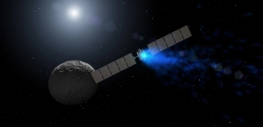
Image: This artist’s rendering shows NASA’s Dawn spacecraft maneuvering above Ceres with its ion propulsion system. Dawn arrived into orbit at Ceres on March 6, 2015, and continues to collect data about the mysterious and fascinating world. The mission celebrated its ninth launch anniversary on September 27, 2016. Credit: NASA/JPL-Caltech/UCLA/MPS/DLR/IDA.

Speaking of Marc Rayman, he deserves great thanks for his efforts at keeping an ongoing chronicle of Dawn operations available in his Dawn Journal. In his latest entry, Rayman notes how he always had to write these entries in haste because of his full schedule, but it’s the mark of a gifted narrator that haste is never an impression the reader comes away with. He has always seemed to be a patient and thorough writer who took the time to get things right.

The last two entries have been cases in point, describing the end of the Dawn mission and what is happening aboard the spacecraft. Immediately ahead is the final act, the loss of hydrazine that will eventually cause Dawn to lose the ability to orient itself — this could occur within weeks — and thus the spacecraft will no longer be able to point its solar panels at the Sun or its radio antenna at Earth (Dawn’s reaction wheels failed earlier in the mission, making hydrazine a critical factor). Radio silence will ensue. What happens next is an interesting question:

We also took a short look at the long-term fate of the spacecraft. To ensure the integrity of possible future exploration that may focus on the chemistry related to life, planetary protection protocols dictate that Dawn not contact Ceres for at least 20 years. Despite being in an orbit that regularly dips so low, the spaceship will continue to revolve around its gravitational master for at least that long and, with very high confidence, for more than 50 years. The terrestrial materials that compose the probe will not contaminate the alien world before another Earth ship could arrive.

So we have a window of about 50 years and perhaps more before Dawn will come down on Ceres, and Rayman’s inference here is that this gives time to mount another mission to Ceres before any contamination could occur. But given that it has also been 50 years since Apollo, I for one don’t necessarily see this as a very large window, and can only hope that its presence will be a motivator for a return to the dwarf planet before we have to wonder whether what we find there could have been affected by anything from Earth.

Dawn is the only spacecraft to orbit a body in the asteroid belt, and it is also the only spacecraft to orbit two extraterrestrial destinations, a feat that was accomplished thanks to its ion propulsion system. Dawn reached the 4.5 billion year old Vesta in 2011 and spent 14 months orbiting it, showing us a mountain at the center of the Rheasilvia basin that turns out to be twice the height of Mt. Everest, along with multiple canyons that fit into Grand Canyon scale. We also learned that Vesta, with its violent history, was the source of a common family of meteorites.

Ceres turned out to be even more of a surprise, with its bright salty deposits made up of sodium carbonate in the form of a slushy brine that originated from below the crust. Some regions on Ceres were geologically active in comparatively recent times, indicating a deep reservoir of liquid. Organic molecules turned up in the area around Ernutet Crater, but we lack the instrumentation aboard the spacecraft to be able to say whether they were formed by any biological processes. “There is growing evidence that the organics in Ernutet came from Ceres’ interior, in which case they could have existed for some time in the early interior ocean,” said Julie Castillo-Rogez, Dawn’s project scientist and deputy principal investigator at JPL.

With its high-resolution images, gamma ray and neutron spectra, infrared spectra, and gravity data, Dawn has delivered full value and continues, as this JPL news release reminds us, to “swoop over Ceres about 22 miles (35 kilometers) from its surface — only about three times the altitude of a passenger jet.” For his part, Marc Rayman thinks about Dawn after it goes silent as “an inert, celestial monument to human creativity and ingenuity,” which it is. But the data Dawn gathered still lives, and will resonate in the form of discoveries and new papers for decades.

Extending the Habitable Zone

Not long ago, Ramses Ramirez (Earth-Life Science Institute, Tokyo) described his latest work on habitable zones to Centauri Dreams readers. Our own Alex Tolley (University of California) now focuses on Dr. Ramirez’ quest for ‘a more comprehensive habitable zone,’ examining classical notions of worlds that could support life, how they have changed over time, and how we can broaden current models. We can see ways, for example, to extend the range of habitable zones at both their outer and inner edges. A look at our assumptions and the dangers implicit in the term ‘Earth-like’ should give us caution as we interpret the new exoplanet detections coming soon through space- and ground-based instruments.

by Alex Tolley

The Plains of Tartarus – Bruce Pennington

In 1993, before we had detected any exoplanets, James Kasting, Daniel Whitmire, and Ray Reynolds published a modeled estimate of the habitable zone in our solar system [1]. They stated:

“A one-dimensional climate model is used to estimate the width of the habitable zone (HZ) around our sun and around other main sequence stars. Our basic premise is that we are dealing with Earth-like planets with CO2/H2O/N2 atmospheres and that habitability requires the presence of liquid water on the planet’s surface. The inner edge of the HZ is determined in our model by the loss of water via photolysis and hydrogen escape. The outer edge of the HZ is determined by the formation of CO2 clouds, which cool a planet’s surface by increasing its albedo and by lowering the convective lapse rate. Conservative estimates for these distances in our own Solar System are 0.95 and 1.37 AU, respectively; the actual width of the present HZ could be much greater. Between these two limits, climate stability is ensured by a feedback mechanism in which atmospheric CO2 concentrations vary inversely with planetary surface temperature. The width of the HZ is slightly greater for planets that are larger than Earth and for planets which have higher N2 partial pressures. The HZ evolves outward in time because the Sun increases in luminosity as it ages. A conservative estimate for the width of the 4.6-Gyr continuously habitable zone (CHZ) is 0.95 to 1.15 AU.”

Climate models have improved considerably over time, and now are capable of three dimensional (3-D) models as well as more advanced 1-D models. Parameter estimations are also being refined to account for different atmospheric features.

The 1993 Kasting et al paper set the bounds for a conservative HZ at 0.95 and 1.37 AU, the outer bound being inside the orbit of Mars. However, the authors noted that a maximal greenhouse with a dense, CO2 atmosphere would push the outer bound to 1.67 AU, that would include Mars, although this was considered optimistic. In 2013, Kopparapu, Ramirez, Kasting, et al, published new estimates on the HZs using a more advanced 1-D model [3]. For the Solar System, the inner and outer edges were 0.99 and 1.67 AU respectively, with the now conservative outer limit at maximal greenhouse warming.

In 2018, Dr. Ramirez published a review of HZ research that included ideas that extended the HZ in time and space, as well as a wider range of stellar types [4]. The conclusion of that paper included the decision tree concerning newly discovered planets and models of their environments. The decisions have identifying numbers added and are shown in figure 1.

In a recent Centauri Dreams essay, Revising the Classical ‘Habitable Zone’, Dr. Ramirez outlined his reasons for studying models of planetary habitable zones (HZ) and environments as part of the search for life. This post will try to tie the many ideas of the journal article to the decision points in figure 1 below.

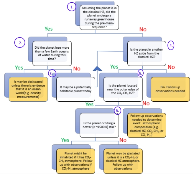
Figure 1. Reproduced from the paper [4], annotated with numbers.

1. Assuming the planet is in the classic HZ, did planet have a runaway GHE during pre-main sequence?

The classic HZ calculates its inner limit as the point at which a runaway greenhouse effect (RGE) can occur. This inner edge is calculated for the period when the star is in the main sequence. For most stars, the main sequence starts quite quickly, within 0.1 Gyr of the nebula forming, allowing life to evolve after the main sequence had started and before the star in its potentially more luminous pre-main sequence state has had time to initiate the RGE. However, for the numerically numerous M-dwarfs, this pre-main sequence period may last for up to a 1 Gyr and have orders of magnitude more luminosity than during the main-sequence. Any planet currently in the classic HZ would have been subject to far higher luminosities and with a time period sufficient to desiccate the planet. The world might then be like Venus, a hot, dry world, with our without a dense CO2 atmosphere. Transit techniques will detect Earth-sized rocky worlds more easily around M-dwarfs, which have attracted a fair amount of discussion about the conditions for life on their surfaces. The issue of a high luminosity during a long pre-main sequence period may trump any favorable conditions during the current main sequence period. Therefore whether the exoplanet lost all of its water during this time needs to be addressed, which leads us to:

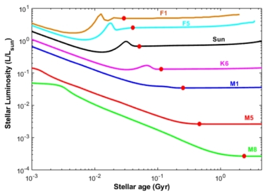
Figure 2. Evolution of stellar luminosity for F – M stars (F1, F5, Sun, K6, M1, M5, and M8) using Barrafe et al. [184] stellar evolutionary models. When the star reaches the main-sequence (red points) the luminosity curve flattens. [4]

2. Did the planet lose more than a few Earth oceans of water during the pre-main sequence period?

An Earth analog planet will desiccate like Venus if it loses more than a few Earth oceans of water. It is possible that the water loss was not severe when the planet entered the classic HZ. If the water loss was high, the world would be desiccated, like Venus.

If any of these conditions are not satisfied:

3. If water loss was not sufficient to desiccate the planet

If the period and intensity of water loss was insufficient to result in a complete RGE, or the starting volume of water was low, then the planet may be characterized as a desert world, with lakes of water, possibly at altitude.

One possibility is that the world is an ocean world with far higher quantities of water than an Earth analog. In this case, desiccation has been held off as a result. Density calculations for that world will indicate if the planet may be an ocean world. As far as life is concerned, we would return to the issue of whether such ocean worlds are suitable for sustaining any abiogenesis derived life.

If the planet has retained enough water it may join the candidates for the next decision: This allows the planet to be considered potentially habitable regardless of early heating.

The author then allows for a wider interpretation of the HZ:

4. Is the planet in another HZ that is outside the classic HZ?

The bulk of the paper deals with possible modifications of the HZ that extend its range at both the inner and outer edges. The paper documents a number of mechanisms that could widen the HZ and to what one might call an optimistic HZ.

Some examples are listed below:

A. Empirical vs model HZs

The author argues that empirical, rather than model limits for the classic HZ might be applied. These limits imply that the outer edge must have been further than the climate model as Mars has evidence that it once had running water on its surface when the sun’s luminosity was lower. For the inner edge, this puts the edge of the HZ closer to the sun at 0.75 AU, but still outside the orbit of Venus as the planet has no sign of surface water even 1 Gya when the sun was cooler [Figure 3].

B. Stellar spectral range

The author argues that the apparent rapid emergence of life on earth allows for hotter, shorter-lived stars to harbor life before they exit the main sequence. This extends the HZ to beyond the star types usually associated with life, but to large, hot stars.

C. Extensions of the HZ in space

Greenhouse gases like methane (CH4) and hydrogen (H2) can extend the HZ, particularly at the outer edge. Methane could extend the HZ beyond Mars, and as it is also produced biologically in greater quantities than geological processes, can maintain the gas in the atmosphere. It is often cited as a detectable gas out of equilibrium and possibly indicative of life. H2 may also contribute to warming and has be posited as a possible explanation for the warmer, ice-free Earth during the Archean.

Ocean worlds are often cited as having unregulatable temperatures due to the absence of exposed crust that prevent the carbon-silicate cycle to act as a carbon sink. One model of ocean worlds with ice caps suggests a way for this sink to operate with CO2 clathrates.

Binary stars would appear to be problematic for worlds to stay in their HZ. The climates are difficult to model, especially where the planet orbits one star, but the planet may create a temporary, benign temperature with periods of freezing as is transits into and out of an HZ.

3-D climate modeling is now increasingly able to compute the effects of rotation rates and different types of cloud cover and composition. The results vary regarding whether these parameters can extend the HZ.

This leads to a sub-question: about the outer edge of the extended HZ:

5. Is the planet near the outer edge of the classic HZ?

The classic HZ outer edge is set by the maximum warming effect of an atmosphere with CO2 and H2O. However, there are some possible ways to extend that outer edge using other greenhouse gases like CH4 and H2. Figure 3 shows the effect of CH4 and H2 on the outer limit of the HZ. For most worlds, retaining a light H2 component to the atmosphere is unlikely, unless it is maintained by some geologic or biotic process. Other possibilities include transient warming periods, possibly even limit cycles that create warm conditions on a periodic basis, perhaps with CH4 or H2 that can exist for short periods. Of course, life would have to survive in some form during the planet’s frozen period. Even on the hypothesized Snowball Earth, liquid water was probably present below the surface ice. For a solidly frozen world, the conditions for survival would be harsher.

For M dwarfs, with high luminosity, and long pre-main sequence periods, planets currently residing at the outer edge of the classic HZ may have been habitable during this pre-main sequence period. Life may have evolved during that period, then retreated to the subsurface as the planet cooled. This is analogous to the hopes of some that life on Mars may have evolved when the planet had surface water, but may still exist at depth as Mars surface cooled and dried.

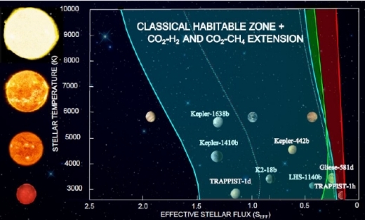
Figure 3. The classical HZ (blue) with CO2-CH4 (green) and CO2-H2 (red) extensions for stars of stellar temperatures between 2,600 and 10,000 K (A – M-stars). Some solar system planets and exoplanets are also shown. [4]

6. Is the planet orbiting a hotter ( >~ 4500 K) star?

Because the star type influences the warming of the atmosphere and planet’s surface, only stars with a surface temperature greater than 4500K will extend the outer edge of the HZ with the greenhouse gas, Ch4, as part of a dense CO2 atmosphere. Unintuitively, for cooler stars, CH4 in the CO2 atmosphere brings the outer limit of the HZ closer to the star. This is clearly shown in Figure 3. [See also CD post The Habitable Zone: The Impact of Methane.] Hydrogen (H2) will quite considerably extend the outer limit of the HZ for all stellar types. Spectroscopy to determine the atmospheric mixing ratios will help in determining whether this is possibly the case.

Other considerations

The paper ignores the current vogue for life in icy moon subsurface oceans for good reason as any subsurface liquid ocean is undetectable by any telescopes that we have on the near horizon. Focusing on the HZ where surface water can exist makes operational sense.

This paper does us a service in not just offering routes to expanding the HZ, but also in the approach to characterizing planets, and ultimately to modeling them accurately once we have the empirical data to support these models.

In passing, the author gives credence to the issues of interpreting results. There is a criticism of the use of “HZ” and “Earth-like” and super-Earth” to imply that those exoplanets have Earth-like life in abundance on their surfaces. In many ways, the extending of HZs retains the concept of surface water possibly existing. In the original Kasting et al paper, their HZ definition required surface water as a necessary condition for life to evolve, as we currently believe. Nevertheless, these worlds may be sterile, as this condition may be insufficient.

As Moore states[5]:

“Habitable planets, not habitable zones Similarly, the term habitable zone is misleading to both the public and the scientific community. On the face of it, habitable-zone planets should be, well, habitable, but in its now classic definition, this is the region in which the presence of a liquid water surface “is not impossible” with an atmosphere assumed to be Earth-like. It does not mean that a habitable zone planet would, in fact, have a wet surface or any other condition required for life. Furthermore, this definition ignores the potential for deep, chemosynthetic biospheres and biases our thinking toward only one of the many ways in which life manages to sustain itself on Earth. That the term habitable zone has such a disconnect with the concept of habitability is problematic for communicating ideas clearly and yet its use has become entrenched in discussions of new exoplanet results and it continues to inform the design of our exoplanet program.”

For life in the Earth’s Archean eon, prokaryotic methanogens create methane (CH4). This greenhouse gas must be present in sufficient quantities to be detected and should push out the inner bound of the HZ.

With these caveats in mind, the Ramirez paper suggests that we can use these expanded HZs to both focus the search for targets, and to validate the models so that targets can be more accurately determined as we extend our searches. This might be very timely as the Transiting Exoplanet Survey Satellite (TESS) all-sky survey is already turning up many potential targets.

References

Kasting, J.; Whitmire, D.; Raynolds, R. “Habitable Zones Around Main Sequence Stars.” Icarus 1993, 101, 108–128.

Kasting, J. How to Find a Habitable Planet. Princeton University Press, 2010.

Kopparapu, R. K.; Ramirez, R.; Kasting, J. F.; Eymet, V.; Robinson, T. D.; Mahadevan, S.; Terrien, R. C.; Domagal-Goldman, S.; Meadows, V.; Deshpande, R. “Habitable Zones Around Main-Sequence Stars: New Estimates.” Astrophys. J. 2013, 765, 131, doi:10.1088/0004-637X/765/2/131.

Ramirez, R M “A more comprehensive habitable zone for finding life on other planets” Geosciences 2018, 8(8), 280.

Moore et al “How habitable zones and super-Earths lead us astray” Nature Astronomy volume 1, Article number: 0043 (2017).

New Horizons: Checking in on Approach Operations

Here’s another, wider look at New Horizons’ view of Ultima Thule (MU69), its next target, which we first saw in late August, though the image was acquired at mid-month. I like this view because it gets across just what a tricky acquisition this was. Look at the background star-field! Consider that Ultima is still 100 times fainter than Pluto as seen from Earth, making it about a million times fainter than a naked eye object. LORRI, the spacecraft’s Long Range Reconnaissance Imager, once again demonstrates its key role in the mission.

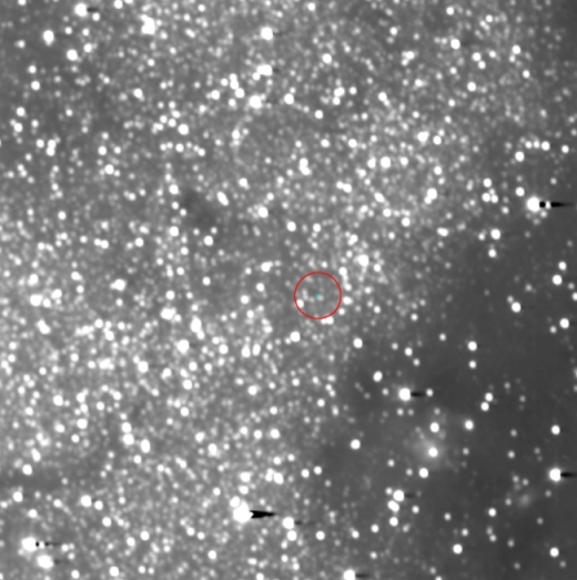
Image: New Horizons spotted Ultima Thule for the first time on August 16, near the center of the red circle in this LORRI image of the dense Milky Way star field where Ultima lies. Credit: JHU/APL.

Getting the image as early as it did was something of a coup for New Horizons, this being the first attempt, made just after the spacecraft transitioned from spin-stabilized mode (during cruise) to pre-flyby mode, which allows its cameras and other instruments to point as needed. According to New Horizons’ PI Alan Stern, the detection images were returned to Earth on August 18-19, where they received the necessary processing to remove artifacts. Says Stern:

Scientists on our team in Maryland, Arizona, and Colorado jumped right onto those data, carefully processing them to remove background stars and other artifacts — and out popped Ultima, a faint beacon, dead ahead, in just the very pixel our navigation crew had predicted it would show up!

Useful work indeed, allowing regular imaging from the spacecraft to refine New Horizons’ course. We learn in Stern’s latest report that the team plans to execute a course correction on October 3, affecting the craft’s trajectory by about 3 meters per second, so the team is already fine-tuning approach and arrival parameters. As part of future course refinements, remember that we now have data from the occultations of a background star by Ultima that occurred on August 3-4, events that were observed by teams in Senegal and Colombia. For more on this and the previous occultation work in Patagonia, see On to Ultima Thule.

We can anticipate a full update from mission scientists at the 50th annual meeting of the Division for Planetary Sciences, coming up in late October in Knoxville, TN, where new results from Pluto/Charon will also be discussed. Right now, the search for collision hazards near Ultima continues as does navigation imaging of the target, which could well lead to future course-corrections. Although no hazardous debris has yet turned up in the occultation data, November and December will see the LORRI instrument scanning the target intensely at closer range. And Ultima Thule isn’t the only KBO in the mix, as Stern reports:

New Horizons will collect data on a half-dozen other Kuiper Belt objects and the plasma and dust environment way out there in the Kuiper Belt, nearly 4 billion miles from Earth. Also, our flight team will be finalizing the software loads to drive the spacecraft’s close-up flyby observations of Ultima and its environment, from geology to composition, to searches for moons, rings and any atmosphere Ultima may sport.

And for another sense of scale, the image below views New Horizons’ current position in relation to the rest of the Solar System. Now would be a good time to read, if you haven’t already, Stern and David Grinspoon’s Chasing New Horizons (Picador, 2018). In the book, the authors discuss how critical pre-flyby planning and maneuvers were to get the spacecraft to arrive at closest approach to Pluto/Charon within the tight window (9 minutes!) necessary for all the spacecraft’s programmed pointing maneuvers to center its targets.

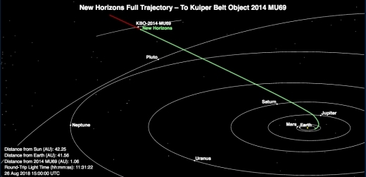
Image: New Horizons has crossed almost all of the 1.6 billion kilometers (1 billion miles) separating the July 14, 2015, flyby of Pluto and the upcoming January 1, 2019, flyby of the Kuiper Belt object (KBO) nicknamed Ultima Thule. Credit: JHU/APL.

What Stern tells Grinspoon here is just as germane to the approach to Ultima Thule:

Much of how New Horizons achieved this goal was done with careful optical navigation and rocket-engine firings that the spacecraft performed to home in on the closest-approach time. But mathematical analysis had shown that this alone might not be good enough to guarantee arrival in the critical plus-or-minus 540 second window. So the spacecraft’s engineers at APL also built in some clever software to correct for any remaining timing errors once it was too late to fire the engines.

The importance of the optical information is likewise clear:

As the spacecraft approached Pluto, every day the optical navigation team used new images to determine just how far off the closest approach timing was going to be, and then calculated the timing knowledge update needed to correct for that. Concurrently, Leslie Young and her encounter planning team used sophisticated software tools to generate a ‘science consequences report,’ in which each close-approach observation was simulated for the newly predicted timing error to determine, assuming no correction was made, which would succeed and which would fail.

For the Ultima Thule encounter, the New Horizons team is conducting mission simulations and working through procedures for over 250 possible spacecraft contingencies should problems arise (as part of that effort, new fault protection software has already been uploaded). With the journey from Pluto/Charon to the KBO now 90 percent complete, we can look forward to the New Year’s Eve flyby, followed by further data acquisition from the Kuiper Belt beyond.

Transiting Debris around a White Dwarf

Who among us hasn’t speculated about the ultimate fate of the Solar System? The thought of our Sun growing into a vast red giant has preoccupied writers and readers since the days when H. G. Wells so memorably captured a far future scene through the eyes of his Time Traveler. And what a scene that was:

“I cannot convey the sense of abominable desolation that hung over the world. The red eastern sky, the northward blackness, the salt dead sea, the stony beach crawling with these foul, slow-stirring monsters, the uniform poisonous-looking green of the lichenous plants, the thin air that hurts one’s lungs: all contributed to an appalling effect. I moved on a hundred years, and there was the same red sun—a little larger, a little duller—the same dying sea, the same chill air, and the same crowd of earthy crustacea creeping in and out among the green weed and the red rocks. And in the westward sky, I saw a curved pale line like a vast new moon.”

Wells was working on a different timescale than we now know to be the case, but we track his protagonist in leaps of a thousand years each as he moves into the future, “…drawn on by the mystery of the earth’s fate, watching with a strange fascination the sun grow larger and duller in the westward sky…” He catches the transit of a planet across the swollen Sun but doesn’t know which it is — so distorted appears the Solar System in the sky above that he wonders if Mercury is not near the Earth in this era, an inner planet imperiled by its own monstrous star.

It’s lively stuff, and demands translation into our current understanding of stellar evolution: What does happen to our system’s planets when the Sun expands to red giant stage? One way of looking into this is to see what we can find around white dwarf stars, the ultimate destinations of stars in the Sun’s mass range after the red giant era ends. At this point, our star will have lost its outer layers, leaving only a comparatively tiny, dense core.

Back in 2015, Andrew Vanderburg (Harvard-Smithsonian Center for Astrophysics) and colleagues published their findings about the white dwarf WD 1145+017, located in Virgo about 570 light years from Earth. The researchers were working with data from the rejuvenated K2 mission, which revealed that light from the star was periodically dimmed by a series of objects. The rocky bodies responsible were, the paper suggested, disintegrating, leaving traces of calcium, iron and aluminium on the white dwarf’s surface.

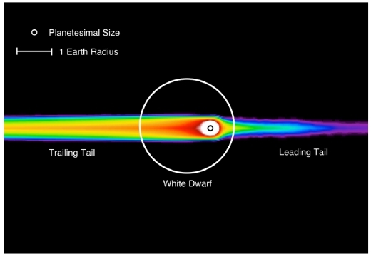
Image: A schematic of the trailing and leading cometary tails from the disintegrating planetesimal compared to the White Dwarf host size. Figure from Vanderburg et al. (2015).

Now we have further insights into the same star from a team led by Paula Izquierdo of the University of La Laguna, Spain, who went to work on the white dwarf using the Gran Telescopio Canarias (GTC) and the Liverpool Telescope (LT). The method was fast optical spectrophotometry and photometry, analyzing the acquired spectra as a function of wavelength. With data from both telescopes, the objects around WD 1145+017 have been captured making two deep transits.

What emerges is that there is a lengthy period between the beginning of the transits and their end, one that is consistent, according to the researchers, with a comet-like tail. This fits with the earlier work of Vanderburg and team, who believed they were seeing the signatures of dust and gas clouds being produced from solid fragments on a roughly 4.5 hour orbital period. Moreover, there is a noteworthy timing feature that the paper explains, with an interesting comparison:

We note in passing that the six times of transit minimum are roughly equally spaced in time, with an average separation of 6.2±1.1 min. The nearly equal spacing of these bodies is reminiscent of the string of fragments of comet Shoemaker-Levy 9 (Weaver et al. 1994).

The famous ‘string of pearls’ comet may thus have an analogue around a distant white dwarf, or else, says the paper, we are seeing evidence of a dense debris cloud, or multiple clouds, extending 120° in azimuth. The authors find that WD 1145+017 has a mass of 0.63 ± 0.05 Solar masses and a cooling age of 224 million years, plus or minus 30 Myr. The ‘cooling age’ is a reference to the white dwarf’s age as a degenerate star; it does not, in other words, include its long span as a main sequence star and the red giant phase that would have followed it.

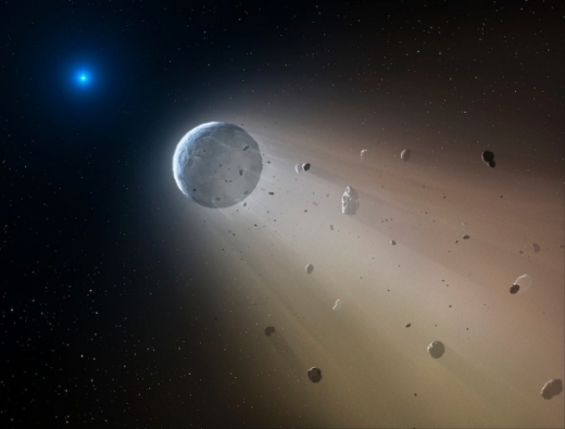
Image: The K2 mission spotted a disintegrating planet swirling around a white dwarf star. Credit: Mark Garlick.

Is this the fate of our own Solar System, to be shredded into clouds of debris around a slowly cooling white dwarf? For decades, we’ve known that the surfaces of some white dwarfs are rich in metals, possible debris from the original system. Now we can push that speculation further, in this case aided by useful transit signatures. This is a lengthy process, as the authors of the Izquierdo study note in relation to WD 1145+017, but one with a clear path for future work:

The decrease in the strength of the circumstellar line provides no information on the relative location of gas and dust along the line-of-sight towards the white dwarf. Time-resolved spectroscopy with a higher signal-to-noise ratio has the potential to provide further insight into the geometry of the gas and dust within WD 1145+017.

The paper is Izquierdo et al., “Fast spectrophotometry of WD 1145+017,” Monthly Notices of the Royal Astronomical Society (24 August 2018). Abstract. The Vanderberg paper is “A disintegrating minor planet transiting a white dwarf,” Nature 526 (22 October 2015) 546-549 (abstract).

‘Rogue’ Planet Population in the Galaxy

We’ve recently looked at gas giant planet formation, and specifically the stages in which Jupiter seems to have formed — this is the work of Thomas Kruijer (University of Münster) and colleagues as summarized in A Three Part Model for Jupiter’s Formation. Whether or not the details of Kruijer and team’s model are correct, it seems evident that gas giants must form quickly, based on current theories. These involve the formation of a large solid core, with gas accretion building up a thick atmosphere at a time when the disk around the parent star is still rich in materials.

In this thinking, planets like the Earth come along much later than the gas giants that are the first to form. Get a few million years into the evolution of a stellar system and there should be evidence of a gas giant, if one is going to form, but terrestrial worlds can take up to 100 million years to emerge. This has captured the interest of Nader Haghighipour (University of Hawaii), whose work was presented at the General Assembly of the IAU meeting in Vienna.

Haghighipour is interested in so-called ‘rogue’ planets, and his focus is on early system formation as a way of exploring their population in the galaxy. Bruce Dorminey has a good entry on this in Forbes, recounting the basics of Haghighipour’s statistical study, one that involved 500 simulations of terrestrial planet formation, including multiple models.

What gets intriguing here is that Haghighipour believes most stellar systems wouldn’t be very good at ejecting planets out of the parent system. This has bearing, of course, on the question of how many rogue planets, free-wandering worlds without a star, might be out there.

It is an issue that is a long, long way from being resolved. Without the reflected light of a primary, such planets are extremely hard to detect except through gravitational lensing, where the light of a background star may be affected by the curvature of spacetime in the presence of a gravitational well, the distortion giving us information about the intermediate object. Used in the exoplanet hunt, gravitational microlensing allows us to spot planets down to rocky, terrestrial-sized worlds around stars thousands of light years away, with the significant limitation that such observations are one-off affairs. You can’t realign the stars to do a second run.

The Microlensing Observations in Astrophysics (MOA) survey, based in New Zealand, as well as the Optical Gravitational Lensing Experiment (OGLE), using a 1.3 meter telescope in Chile, have found a small number of possible ‘rogue’ planets of roughly Jupiter’s mass. A 2011 paper made the case that given microlensing probabilities — and taking into account the efficiency of the equipment at these installations and the rate of such lensing — there could be as many rogue planets in the Milky Way as there are stars. Louis Strigari (Stanford University) has likewise estimated high numbers of rogue planets ranging from Ceres-size on up to gas giants.

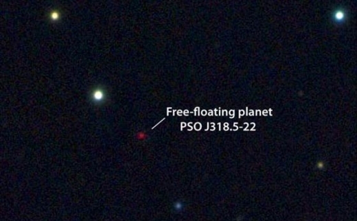
Image: One apparent free-floating planet turned up in a search for brown dwarfs. This multicolor image is from the Pan-STARRS1 telescope, showing PSO J318.5-22, in the constellation of Capricornus. The planet is extremely cold and faint, about 100 billion times fainter in optical light than the planet Venus. Most of its energy is emitted at infrared wavelengths. The image is 125 arcseconds on a side. Credit: N. Metcalfe & Pan-STARRS 1 Science Consortium.

But at the same IAU meeting, according to Dorminey’s report, Yutong Shan (Harvard University) presented evidence from the K2 mission, using data from both the revived Kepler and ground-based surveys. Shan’s team was hunting for free-floating planets, but while they found candidates, none were conclusive — in other words, the detections may be brown dwarfs.

For his part, Nader Haghighipour believes that there aren’t as many rogue planets to find as some believe. The reason: It’s when the protoplanetary disk is seething with youthful energies that planets are likely to be ejected — few terrestrial worlds available then — and only 1-2 percent of these would leave the system. Shan’s Kepler study is ongoing, but as Dorminey notes, the early results seem to support Haghighipour in his doubts over rogue planet ejections.

But we are early in this work. Let me also draw your attention to work at the University of Oklahoma from Xinyu Dai and Eduardo Guerras. Working with data from the Chandra X-Ray Observatory and microlensing models of their own design, the duo have been studying the black hole at the center of quasar RX J1131–1231. Here we have a background quasar being lensed by the foreground black hole, and Dai and Guerras show that these emissions near the Schwarzschild radius of the black hole can be affected by planets nearby in its galaxy.

What we get here is another ‘rough cut’ at rogue planets, this time in another galaxy, and in it, the authors calculate about 2000 objects per main sequence star, in sizes ranging from the Moon to Jupiter. Dai and Guerras, in other words, come up with numbers that come closer to supporting Strigari than Haghighipour. All of which makes a strong case that on the subject of rogue planets in this or any galaxy, what we still don’t know vastly outweighs what we do.

The microlensing paper mentioned above is Sumi et al., “Unbound or distant planetary mass population detected by gravitational microlensing,” Nature 473 (19 May 2011), 349-352 (abstract). The Strigari paper is “Nomads of the Galaxy” Monthly Notices of the Royal Astronomical Society Vol. 423, Issue 2 (21 June 2012 – abstract). The paper on RX J1131–1231 is Xinyu Dai & Eduardo Guerras, “Probing Planets in Extragalactic Galaxies Using Quasar Microlensing,” Astrophysical Journal Letters Vol. 853, No. 2 (2 February 2018). Abstract.

Finding Jupiter’s Water

One of the memorable things about 1995 (and this was also the year of the first detection of an exoplanet around a main sequence star) was the release of the Galileo spacecraft’s descent probe. Dive into that howling maelstrom, it would seem, and instant obliteration should follow. But the probe had been designed with a heavy duty heat shield to protect it during its journey. It kept transmitting after scorching its way into Jupiter’s atmosphere at 47 kilometers per second, 30 km/sec faster than Voyager 1. The probe returned data for fully 58 minutes before its demise.

Here’s how two science fiction novelists handle a descent into the Jovian clouds:

Slowly, the fine fretwork of the ammonia cirrus clouds above him became obscured by brown and salmon layers of intervening chemistry, the air stained a nicotine-coloured haze of complex carbon molecules. Soon it was warmer than a summer’s day out there, and already the gondola was enduring more than ten atmospheres of pressure, the structure making slight creaking sounds as it absorbed the mounting forces. Falcon eyed the hull around him with a certain wariness, trusting that the Kon-Tiki’s molecular-scale refurbishments had been as thorough as claimed.

A certain wariness seems justified. And this:

Overhead, the sky was darkening through shades of purple. This was not the onset of evening — dusk was still hours away — but the gradual filtering out of solar illumination. Much the same thing happened in the depths of Earth’s oceans. The main difference here was that the external temperature was steadily rising, even as the iron crush of the atmosphere redoubled its hold on the gondola.

That’s Stephen Baxter and Alastair Reynolds in The Medusa Chronicles (Saga, 2016), which picks up on Arthur C. Clarke’s 1971 novella “A Meeting with Medusa,” and takes its hero into the heart of Jupiter, the earliest part of which descent is glimpsed in the paragraph above. Doubtless Baxter and Reynolds were all over the Galileo data as they made the transition between what we know to the ingenious plot they constructed. Galileo’s data had their share of surprises, showing us, for example, stronger winds than expected, but that was just a start for the adventures of the book’s hero.

Let’s leave science fiction for the moment, though I’ll come back to it. The region the Galileo probe descended through turned out to be drier than expected, another Galileo surprise given that ice is the primary constituent of Jupiter’s moons. Now we have new work delving into the question of water on Jupiter. A team led by Gordon Bjoraker (NASA Ames), working with collaborators at several US universities, suggests in a paper in The Astronomical Journal that water is detectable and it may be out there in large quantities indeed.

While Jupiter’s atmosphere is 99 percent hydrogen and helium, it could still contain many times the amount of water we have on Earth. The scientists probed the question using data gathered by ground-based telescopes to detect traces of water deep within Jupiter’s Great Red Spot, working with the iSHELL spectrograph at the NASA Infrared Telescope Facility and the Near Infrared Spectrograph on the Keck 2 telescope (both instruments are at Mauna Kea in Hawaii):

In this paper we present ground-based observations of Jupiter’s Great Red Spot between 4.6 and 5.4 µm. The 5-µm region is a window to the deep atmosphere of Jupiter because of a minimum in opacity due to H2 and CH4. This spectrum provides a wealth of information about the gas composition and cloud structure of the troposphere. Jupiter’s 5-µm spectrum is a mixture of scattered sunlight and thermal emission that varies significantly between Hot Spots and low-flux regions such as the Great Red Spot.

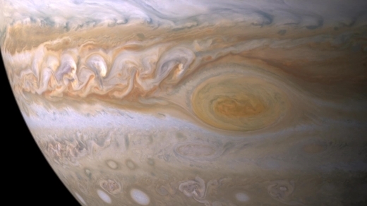
Image: Trapped between two jet streams, the Great Red Spot is an anticyclone swirling around a center of high atmospheric pressure that makes it rotate in the opposite sense of hurricanes on Earth. Credit: NASA/JPL/Space Science Institute.

The Great Red Spot is an enormous storm that, though mutable, has continued to rage for at least 150 years and perhaps much longer than that. The researchers found evidence of three layers of clouds here, with the deepest at 5-7 bars (1 bar approximates the average atmospheric pressure at sea level on Earth). This would be about 160 kilometers below the cloud tops in a region where temperature is thought to reach the freezing point of water. The Bjoraker team describes an opaque cloud layer detected at around 5 bars as ‘almost certainly a water cloud.’

What’s crucial here is the methodology, because if the methods used on the Great Red Spot can be validated by the Juno spacecraft, we can apply them to other gas giants. Now orbiting Jupiter until 2021 and conducting its own search for water using its infrared spectrometer, Juno has as a key objective the identification and characterization of atmospheric H2O, although observations using the spacecraft’s Microwave Radiometer are tricky given the low microwave absorptivity of H2O gas when compared to ammonia.

Thus we have a necessary synergy between ground-based measurements of both H2O and NH3 to support what Juno’s MWR instrument finds and to increase the accuracy of its calibration. This Clemson University news release explains that within months, the team will be collecting ‘many gigabytes’ of data with the iSHELL spectrograph that can be matched against further Juno observations, with a suite of automated software being built to analyze the results.

Getting a better picture of Jupiter’s water content could prove useful in a number of ways, and might even take us in a science fictional direction, says Clemson University co-author Máté Ádámkovics:

“The discovery of water on Jupiter using our technique is important in many ways. Our current study focused on the red spot, but future projects will be able to estimate how much water exists on the entire planet. Water may play a critical role in Jupiter’s dynamic weather patterns, so this will help advance our understanding of what makes the planet’s atmosphere so turbulent.”

True enough. And this takes us back into the imaginative realm of Clarke, Baxter and Reynolds:

“And, finally, where there’s the potential for liquid water, the possibility of life cannot be completely ruled out. So, though it appears very unlikely, life on Jupiter is not beyond the range of our imaginations.”

For those wanting to explore notions of life within Jupiter’s atmosphere, have a look at Larry Klaes’ fine essay Edwin Salpeter and the Gasbags of Jupiter, which looks at a Cornell University collaborator of Carl Sagan and the duo’s unusual musings on a Jovian taxonomy.

The paper is Bjoraker et al., “The Gas Composition and Deep Cloud Structure of Jupiter’s Great Red Spot,” The Astronomical Journal Vol. 156, No. 3 (abstract).

An Asteroid’s Tumultuous Evolution

How extraordinary that we can sometimes tell so much from so little. Extraordinary too how careful we must be to make sure we’re not reading too much into small sample sizes. All of which brings me to the Japanese Hayabusa probe, a spacecraft that survived continual mischance on its journey to asteroid 25143 Itokawa, but was somehow able to return tiny grains of surface material to Earth. And using those materials, scientists are now revealing a violent past that tells us something not only about how the asteroid formed but what happened to it long after.

The work of Kentaro Terada (Osaka University) and colleagues, the investigation follows a complicated path back to the earliest era of our system. But let’s start with the sample collection, which almost didn’t happen: Already damaged from a major solar flare not long after liftoff on May 9, 2003, Hayabusa (the word means ‘falcon’ in Japanese) would also lose two of its three stabilizing reaction wheels. And when the command to deploy its Minerva mini-lander was given, the rover was lost.

Amidst these problems, JAXA (the Japanese space agency) scientists were finally able to bring the spacecraft into contact with the surface, enough so to disturb dust grains it could store for return to Earth. This would mark the first time the surface of an asteroid could be examined in the laboratory, and a decade of this investigation is yielding insights.

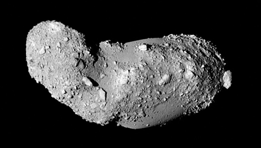
Image: The Hayabusa mission returned samples from Itokawa which are giving clues to the ancient history of the unusual asteroid. Image credit: ISAS, JAXA.

Scientists haven’t had a lot of material to work with, but it doesn’t take much. Examining micrometer-sized phosphate minerals using X-ray micro-tomography, the researchers have been able to perform isotope analysis of uranium (U) and lead (Pb), the latter enabled by Secondary Ion Mass Spectrometry (SIMS). This technique uses a focused ion beam on solid surfaces that causes the ejection of secondary ions that can be measured, revealing their molecular composition. Here’s how lead author Kentaro Terada explains the methods:

“By combining two U decay series, 238U-206Pb (with a half-life of 4.47 billion years) and 235U-207Pb (with a half-life of 700 million years), using four Itokawa particles, we clarified that phosphate minerals crystalized during a thermal metamorphism age (4.64±0.18 billion years ago) of Itokawa’s parent body, experiencing shock metamorphism due to a catastrophic impact event by another body 1.51±0.85 billion years ago.”

Itokawa was indeed formed some 4.6 billion years ago, in the formation period of the Solar System, but we also learn here that its subsequent life has been anything but serene. The second event Terada refers to would likely have been a collision with another asteroid.

Useful here is the comparison between the Itokawa particles and the composition of LL (Low (total) iron, Low metal) chondrites that fall to Earth. This work shows that the formation of Itokawa’s parent body was similar to that of typical LL chondrites — their mineralogy and geochemistry bear strong resemblances — but the collision history of Itokawa, with a catastrophic event 1.4 billion years ago, is significantly different from the ‘shock’ ages of most LL chondrites. The Itokawa shock history resembles, in fact, that of the Chelyabinsk meteorite.

The team goes deeper still, as witness this from the paper:

The observation of a deceleration in the rotation rate of Itokawa also constrains Itokawa’s evolution to within the last 0.1–0.4 million years during which period the conjunction of the two parts referred to as “head” and “body” by a low velocity impact occurred. This conjunction must have occurred after the disruption event and the subsequent main re-accumulation and possibly while the Itokawa fragments still resided within the main belt.

Itokawa was, in other words, pulverized by the collision revealed in these data, eventually reforming into the object we study today over a period of time. Following several billion years in the main asteroid belt, Itokawa was ejected by gravitational resonances into its current Earth-crossing orbit. Drawing on previous work on Itokawa orbits, the authors predict that at some point within the next million years, the asteroid will collide with Earth or else break apart.

Image: Back-scattered electron images of the Itokawa particles. (A–C) Show back-scattered images of polished sections of RA-QD02-0056, RA-QD02-0031, RB-QD04-0025, respectively. (D) Shows the “simulated” slice image of RB-CV-0025 before polishing, based on X-ray microtomography. Here, the angle and depth are selected where the cross sections inside two phosphates become the largest. (E) Shows the “actual” microscope image after careful manual polishing. Most phosphate grains are on the order of 2 µm × 4 µm to 4 µm × 5 µm in size. Credit: Terada et al.

Much rides here on the analysis of a very small amount of material, as the paper is quick to add:

…we emphasize that our successful chronology results for Itokawa are based on a single brecciated particle, RA-QD02–0056, that includes several apatite grains. Such a brecciated grain is so fragile that it may not have been collected if the Hayabusa spacecraft sampling mechanism had operated as planned and its impactors struck the Itokawa surface.

We learn, however, that the Hayabusa team has found other particles that may include phosphorus materials, so further studies should put tighter constraints on the violent events of Itokawa’s evolution.

The paper is Terada et al., “Thermal and impact histories of 25143 Itokawa recorded in Hayabusa particles,” Scientific Reports 8, published 7 August 2018 (full text).

A Glimpse of Ultima Thule

This morning we have an image of MU69, the Kuiper Belt object to which New Horizons is heading, with arrival and flyby scheduled for January 1, 2019. This just after the first glimpse of the asteroid Bennu by the spacecraft now heading there for observation and sample return, OSIRIS-REx. By way of comparison, the first glimpse New Horizons had of Pluto/Charon came during an optical navigation test using the Long Range Reconnaissance Imager (LORRI), which occurred in September of 2006 when Pluto was still 4.2 billion kilometers away.

We knew in the year of its launch, in other words, that New Horizons could find and track targets at extremely long range, but MU69, otherwise known as Ultima Thule, is a tiny target indeed. Moreover, it’s one that raises a host of obstacles particularly in terms of the background stars. We are trying to pluck it out of field objects from a distance of 172 million kilometers.

“The image field is extremely rich with background stars, which makes it difficult to detect faint objects,” said Hal Weaver, New Horizons project scientist and LORRI principal investigator from the Johns Hopkins Applied Physics Laboratory in Laurel, Maryland. “It really is like finding a needle in a haystack. In these first images, Ultima appears only as a bump on the side of a background star that’s roughly 17 times brighter, but Ultima will be getting brighter – and easier to see – as the spacecraft gets closer.”

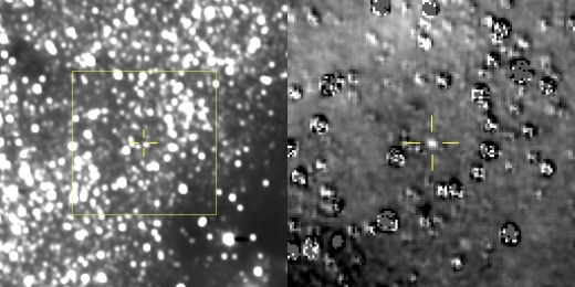
Image: The figure on the left is a composite image produced by adding 48 different exposures from the News Horizons Long Range Reconnaissance Imager (LORRI), each with an exposure time of 29.967 seconds, taken on Aug. 16, 2018. The predicted position of the Kuiper Belt object nicknamed Ultima Thule is at the center of the yellow box, and is indicated by the yellow crosshairs, just above and left of a nearby star that is approximately 17 times brighter than Ultima.

At right is a magnified view of the region in the yellow box, after subtraction of a background star field “template” taken by LORRI in September 2017 before it could detect the object itself. Ultima is clearly detected in this star-subtracted image and is very close to where scientists predicted, indicating to the team that New Horizons is being targeted in the right direction. The many artifacts in the star-subtracted image are caused either by small mis-registrations between the new LORRI images and the template, or by intrinsic brightness variations of the stars. At the time of these observations, Ultima Thule was 172 million kilometers (107 million miles) from the New Horizons spacecraft and 6.5 billion kilometers (4 billion miles) from the Sun. Credit: NASA/Johns Hopkins University Applied Physics Laboratory/Southwest Research Institute.

We are now in the process of continually setting records. These images are the most distant ever taken from the Sun, an honor that was once held by Voyager 1 in its famous ‘Pale Blue Dot’ image of the Earth, taken in 1990. New Horizons likewise snagged the award for most distant image from Earth in December of 2017. The images above were taken on August 16, a series of 48 that succeeded at the spacecraft’s first attempt to find MU69 with its own cameras. Now we can spend the next four months updating the record and watching MU69 grow.

And since ‘first glimpse’ images seem to define this week, here’s that first New Horizons image of Pluto.

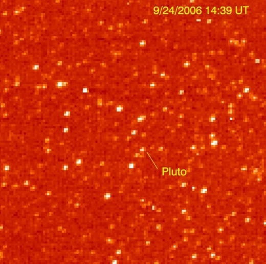
Image: The Long Range Reconnaissance Imager (LORRI) on New Horizons acquired images of the Pluto field three days apart in late September 2006, in order to see Pluto’s motion against a dense background of stars. LORRI took three frames at 1-second exposures on both Sept. 21 and Sept. 24. Because it moved along its predicted path, Pluto was detected in all six images. The images appear pixelated because they were obtained in a mode that compensates for the drift in spacecraft pointing over long exposure times. Credit: NASA/Johns Hopkins University Applied Physics Laboratory/Southwest Research Institute.

This far away from home, it seems fitting to quote from the one Edgar Allen Poe verse, ‘Dreamland,’ that mentions Ultima Thule in its incarnation as a literary figure for the most distant of Earthly places:

By a route obscure and lonely,

Haunted by ill angels only,

Where an Eidolon, named Night,

On a black throne reigns upright,

I have reached these lands but newly

From an ultimate dim Thule –

From a wild weird clime, that lieth, sublime,

Out of Space – out of Time.