Nicole Yunger Halpern's Blog, page 5

The Noncommuting-Charges World Tour (Part 1 of 4)

Introduction: “Once Upon a Time”…with a twist

Thermodynamics problems have surprisingly many similarities with fairy tales. For example, most of them begin with a familiar opening. In thermodynamics, the phrase “Consider an isolated box of particles” serves a similar purpose to “Once upon a time” in fairy tales—both serve as a gateway to their respective worlds. Additionally, both have been around for a long time. Thermodynamics emerged in the Victorian era to help us understand steam engines, while Beauty and the Beast and Rumpelstiltskin, for example, originated about 4000 years ago. Moreover, each conclude with important lessons. In thermodynamics, we learn hard truths such as the futility of defying the second law, while fairy tales often impart morals like the risks of accepting apples from strangers. The parallels go on; both feature archetypal characters—such as wise old men and fairy godmothers versus ideal gases and perfect insulators—and simplified models of complex ideas, like portraying clear moral dichotomies in narratives versus assuming non-interacting particles in scientific models.

Of all the ways thermodynamic problems are like fairytale, one is most relevant to me: both have experienced modern reimagining. Sometimes, all you need is a little twist to liven things up. In thermodynamics, noncommuting conserved quantities, or charges, have added a twist.

Unfortunately, my favourite fairy tale, ‘The Hunchback of Notre-Dame,’ does not start with the classic opening line ‘Once upon a time.’ For a story that begins with this traditional phrase, ‘Cinderella’ is a great choice.

First, let me recap some of my favourite thermodynamic stories before I highlight the role that the noncommuting-charge twist plays. The first is the inevitability of the thermal state. For example, this means that, at most times, the state of most sufficiently small subsystem within the box will be close to a specific form (the thermal state).

The second is an apparent paradox that arises in quantum thermodynamics: How do the reversible processes inherent in quantum dynamics lead to irreversible phenomena such as thermalization? If you’ve been keeping up with Nicole Yunger Halpern‘s (my PhD co-advisor and fellow fan of fairytale) recent posts on the eigenstate thermalization hypothesis (ETH) (part 1 and part 2) you already know the answer. The expectation value of a quantum observable is often comprised of a sum of basis states with various phases. As time passes, these phases tend to experience destructive interference, leading to a stable expectation value over a longer period. This stable value tends to align with that of a thermal state’s. Thus, despite the apparent paradox, stationary dynamics in quantum systems are commonplace.

The third story is about how concentrations of one quantity can cause flows in another. Imagine a box of charged particles that’s initially outside of equilibrium such that there exists gradients in particle concentration and temperature across the box. The temperature gradient will cause a flow of heat (Fourier’s law) and charged particles (Seebeck effect) and the particle-concentration gradient will cause the same—a flow of particles (Fick’s law) and heat (Peltier effect). These movements are encompassed within Onsager’s theory of transport dynamics…if the gradients are very small. If you’re reading this post on your computer, the Peltier effect is likely at work for you right now by cooling your computer.

What do various derivations of the thermal state’s forms, the eigenstate thermalization hypothesis (ETH), and the Onsager coefficients have in common? Each concept is founded on the assumption that the system we’re studying contains charges that commute with each other (e.g. particle number, energy, and electric charge). It’s only recently that physicists have acknowledged that this assumption was even present.

This is important to note because not all charges commute. In fact, the noncommutation of charges leads to fundamental quantum phenomena, such as the Einstein–Podolsky–Rosen (EPR) paradox, uncertainty relations, and disturbances during measurement. This raises an intriguing question. How would the above mentioned stories change if we introduce the following twist?

“Consider an isolated box with charges that do not commute with one another.” 

This question is at the core of a burgeoning subfield that intersects quantum information, thermodynamics, and many-body physics. I had the pleasure of co-authoring a recent perspective article in Nature Reviews Physics that centres on this topic. Collaborating with me in this endeavour were three members of Nicole’s group: the avid mountain climber, Billy Braasch; the powerlifter, Aleksander Lasek; and Twesh Upadhyaya, known for his prowess in street basketball. Completing our authorship team were Nicole herself and Amir Kalev.

To give you a touchstone, let me present a simple example of a system with noncommuting charges. Imagine a chain of qubits, where each qubit interacts with its nearest and next-nearest neighbours, such as in the image below.

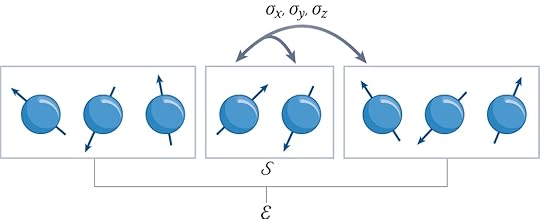The figure is courtesy of the talented team at Nature. Two qubits form the system S of interest, and the rest form the environment E. A qubit’s three spin components, σa=x,y,z, form the local noncommuting charges. The dynamics locally transport and globally conserve the charges.

In this interaction, the qubits exchange quanta of spin angular momentum, forming what is known as a Heisenberg spin chain. This chain is characterized by three charges which are the total spin components in the x, y, and z directions, which I’ll refer to as Qx, Qy, and Qz, respectively. The Hamiltonian H conserves these charges, satisfying [H, Qa] = 0 for each a, and these three charges are non-commuting, [Qa, Qb] ≠ 0, for any pair a, b ∈ {x,y,z} where a≠b. It’s noteworthy that Hamiltonians can be constructed to transport various other kinds of noncommuting charges. I have discussed the procedure to do so in more detail here (to summarize that post: it essentially involves constructing a Koi pond).

This is the first in a series of blog posts where I will highlight key elements discussed in the perspective article. Motivated by requests from peers for a streamlined introduction to the subject, I’ve designed this series specifically for a target audience: graduate students in physics. Additionally, I’m gearing up to defending my PhD thesis on noncommuting-charge physics next semester and these blog posts will double as a fun way to prepare for that.

Colliding the familiar and the anti-familiar at CERN

The most ingenious invention to surprise me at CERN was a box of chocolates. CERN is a multinational particle-physics collaboration. Based in Geneva, CERN is famous for having “the world’s largest and most powerful accelerator,” according to its website. So a physicist will take for granted its colossal magnets, subatomic finesse, and petabytes of experimental data. 

But I wasn’t expecting the chocolates.

In the main cafeteria, beside the cash registers, stood stacks of Toblerone. Sweet-tooth owners worldwide recognize the yellow triangular prisms stamped with Toblerone’s red logo. But I’d never seen such a prism emblazoned with CERN’s name. Scientists visit CERN from across the globe, and probably many return with Swiss-chocolate souvenirs. What better way to promulgate CERN’s influence than by coupling Switzerland’s scientific might with its culinary?1

I visited CERN last November for Sparks!, an annual public-outreach event. The evening’s speakers and performers offer perspectives on a scientific topic relevant to CERN. This year’s event highlighted quantum technologies. Physicist Sofia Vallecorsa described CERN’s Quantum Technology Initiative, and IBM philosopher Mira Wolf-Bauwens discussed ethical implications of quantum technologies. (Yes, you read that correctly: “IBM philosopher.”) Dancers Wenchi Su and I-Fang Lin presented an audiovisual performance, Rachel Maze elucidated government policies, and I spoke about quantum steampunk. 

Around Sparks!, I played the physicist tourist: presented an academic talk, descended to an underground detector site, and shot the scientific breeze with members of the Quantum Technology Initiative. (What, don’t you present academic talks while touristing?) I’d never visited CERN before, but much of it felt eerily familiar. 

A theoretical-physics student studies particle physics and quantum field theory (the mathematical framework behind particle physics) en route to a PhD. CERN scientists accelerate particles to high speeds, smash them together, and analyze the resulting debris. The higher the particles’ initial energies, the smaller the debris’s components, and the more elementary the physics we can infer. CERN made international headlines in 2012 for observing evidence of the Higgs boson, the particle that endows other particles with masses. As a scientist noted during my visit, one can infer CERN’s impact from how even Auto World (if I recall correctly) covered the Higgs discovery. Friends of mine process data generated by CERN, and faculty I met at Caltech helped design CERN experiments. When I mentioned to a colleague that I’d be flying to Geneva, they responded, “Oh, are you visiting CERN?” All told, a physicist can avoid CERN as easily as one can avoid the Panama Canal en route from the Atlantic Ocean to the Pacific through South America. So, although I’d never visited, CERN felt almost like a former stomping ground. It was the details that surprised me.

Familiar book, new (CERN) bookstore.

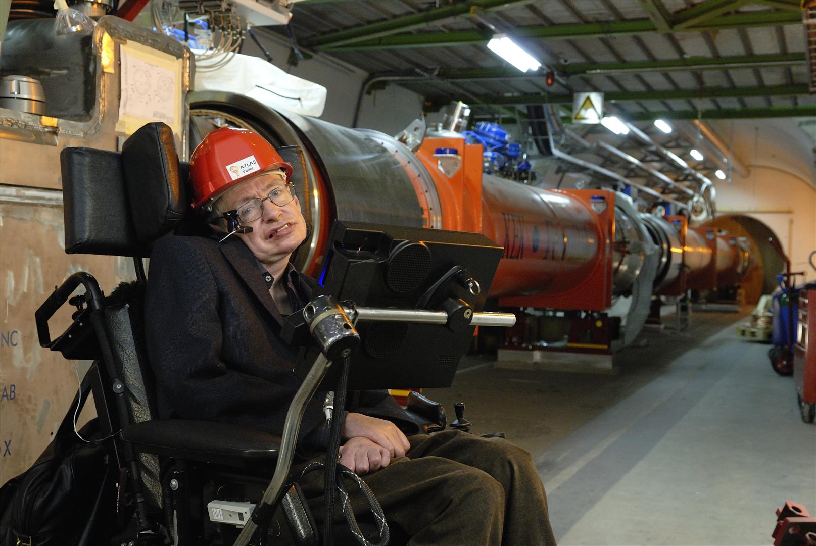
Take the underground caverns. CERN experiments take place deep underground, where too few cosmic rays reach to muck with observations much. I visited the LHCb experiment, which spotlights a particle called the “beauty quark” in Europe and the less complimentary “bottom quark” in the US. LHCb is the first experiment that I learned has its own X/Twitter account. Colloquia (weekly departmental talks at my universities) had prepared me for the 100-meter descent underground, for the hard hats we’d have to wear, and for the detector many times larger than I.

A photo of the type bandied about in particle-physics classes A less famous hard-hat photo, showing a retired detector’s size.

But I hadn’t anticipated the bright, single-tone colors. Between the hard hats and experimental components, I felt as though I were inside the Google logo.

Or take CERN’s campus. I wandered around it for a while before a feeling of nostalgia brought me up short: I was feeling lost in precisely the same way in which I’d felt lost countless times at MIT. Numbers, rather than names, label both MIT’s and CERN’s buildings. Somebody must have chosen which number goes where by throwing darts at a map while blindfolded. Part of CERN’s hostel, building 39, neighbors buildings 222 and 577. I shouldn’t wonder to discover, someday, that the CERN building I’m searching for has wandered off to MIT.

Part of the CERN map. Can you explain it?

Between the buildings wend streets named after famous particle physicists. I nodded greetings to Einstein, Maxwell, Democritus (or Démocrite, as the French Swiss write), and Coulomb. But I hadn’t anticipated how much civil engineers venerate particle physicists. So many physicists did CERN’s designers stuff into walkways that the campus ran out of streets and had to recycle them. Route W. F. Weisskopf turns into Route R. P. Feynman at a…well, at nothing notable—not a fork or even a spoon. I applaud the enthusiasm for history; CERN just achieves feats in navigability that even MIT hasn’t.

The familiar mingled with the unfamiliar even in the crowd on campus. I was expecting to recognize only the personnel I’d coordinated with electronically. But three faces surprised me at my academic talk. I’d met those three physicists through different channels—a summer school in Malta, Harvard collaborators, and the University of Maryland—at different times over the years. But they happened to be visiting CERN at the same time as I, despite their not participating in Sparks! I’m half-reminded of the book Roughing It, which describes how Mark Twain traveled the American West via stagecoach during the 1860s. He ran into a long-lost friend “on top of the Rocky Mountains thousands of miles from home.” Exchange “on top of the Rockies” for “near the Alps” and “thousands of miles” for “even more thousands of miles.”

CERN unites physicists. We learn about its discoveries in classes, we collaborate on its research or have friends who do, we see pictures of its detectors in colloquia, and we link to its science-communication pages in blog posts. We respect CERN, and I hope we can be forgiven for fondly poking a little fun at it. So successfully has CERN spread its influence, I felt a sense of recognition upon arriving. 

I didn’t buy any CERN Toblerones. But I arrived home with 4.5 pounds of other chocolates, which I distributed to family and friends, the thermodynamics lunch group I run at the University of Maryland, and—perhaps most importantly—my research group. I’ll take a leaf out of CERN’s book: to hook students on fundamental physics, start early, and don’t stint on the sweets.

With thanks to Claudia Marcelloni, Alberto Di Meglio, Michael Doser, Antonella Del Rosso, Anastasiia Lazuka, Salome Rohr, Lydia Piper, and Paulina Birtwistle for inviting me to, and hosting me at, CERN.

1After returning home, I learned that an external company runs CERN’s cafeterias and that the company orders and sells the Toblerones. Still, the idea is brilliant.

What geckos have to do with quantum computing

When my brother and I were little, we sometimes played video games on weekend mornings, before our parents woke up. We owned a 3DO console, which ran the game Gex. Gex is named after its main character, a gecko. Stepping into Gex’s shoes—or toe pads—a player can clamber up walls and across ceilings. 

I learned this month how geckos clamber, at the 125th Statistical Mechanics Conference at Rutgers University. (For those unfamiliar with the field: statistical mechanics is a sibling of thermodynamics, the study of energy.) Joel Lebowitz, a legendary mathematical physicist and nonagenarian, has organized the conference for decades. This iteration included a talk by Kanupriya (Kanu) Sinha, an assistant professor at the University of Arizona. 

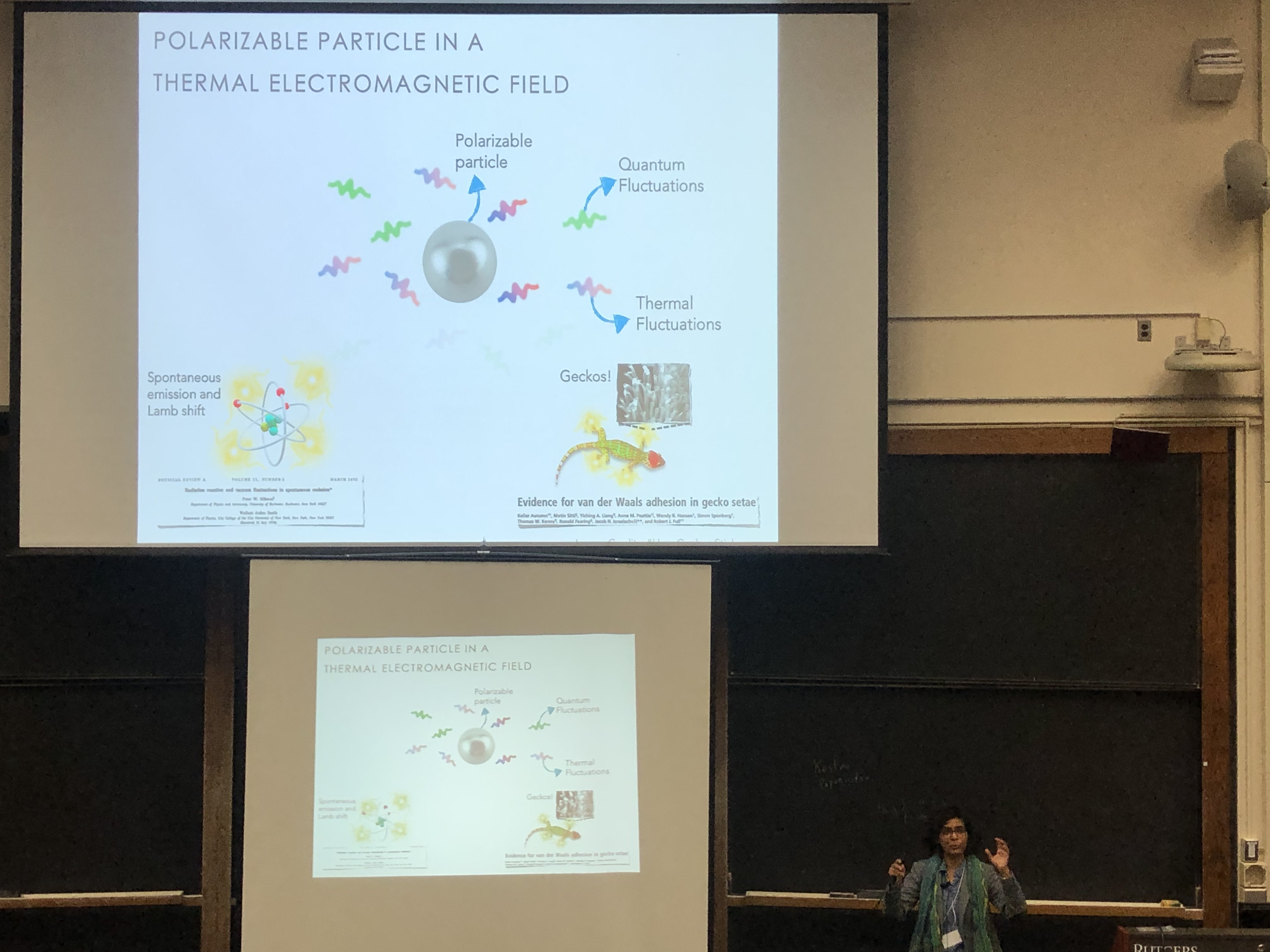
Kanu studies open quantum systems, or quantum systems that interact with environments. She often studies a particle that can be polarized. Such a particle carries an electric charge, which can be distributed unevenly across the particle. Examples include a water molecule. As encoded in its chemical symbol, H2O, a water molecule consists of two hydrogen atoms and one oxygen atom. The oxygen attracts the molecule’s electrons more strongly than the hydrogen atoms do. So the molecule’s oxygen end carries a negative charge, and the hydrogen ends carry positive charges.1

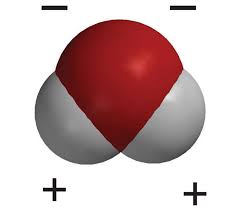The red area represents the oxygen, and the gray areas represent the hydrogen atoms. Image from the American Chemical Society.

When certain quantum particles are polarized, we can control their positions using lasers. After all, a laser consists of light—an electromagnetic field—and electric fields influence electrically charged particles’ movements. This control enables optical tweezers—laser beams that can place certain polarizable atoms wherever an experimentalist wishes. Such atoms can form a quantum computer, as John Preskill wrote in a blog post on Quantum Frontiers earlier this month.

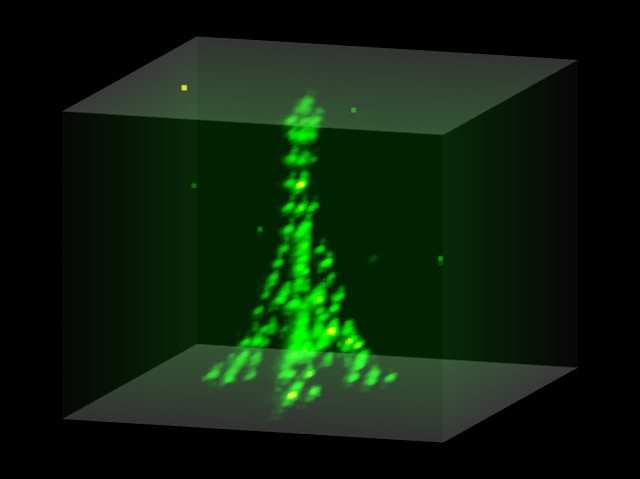Instead of placing polarizable atoms in an array that will perform a quantum computation, you can place the atoms in an outline of the Eiffel Tower. Image from Antoine Browaeys’s lab.

A tweezered atom’s environment consists not only of a laser, but also everything else around, including dust particles. Undesirable interactions with the environment deplete an atom of its quantum properties. Quantum information stored in the atom leaks into the environment, threatening a quantum computer’s integrity. Hence the need for researchers such as Kanu, who study open quantum systems.

Kanu illustrated the importance of polarizable particles in environments, in her talk, through geckos. A gecko’s toe pads contain tiny hairs that polarize temporarily. The electric charges therein can be attracted to electric charges in a wall. We call this attraction the van der Waals force. So Gex can clamber around for a reason related to why certain atoms suit quantum computing.

Kanu explaining how geckos stick.

Winter break offers prime opportunities for kicking back with one’s siblings. Even if you don’t play Gex (and I doubt whether you do), behind your game of choice may lie more physics than expected.

1Water molecules are polarized permanently, whereas Kanu studies particles that polarize temporarily.

You can win Tic Tac Toe, if you know quantum physics.

Note: Oliver Zheng is a senior at University High School, Irvine CA. He has been working on AI players for quantum versions of Tic Tac Toe under the supervision of Dr. Spiros Michalakis.

Several years ago, while scrolling through YouTube, I came across a video of Paul Rudd playing something called “Quantum Chess.” I had no idea what it was, nor did I know that it would become one of the most gloriously nerdy rabbit holes I would ever fall into (see: 5D Chess with Multiverse Time Travel).

Over time, I tried to teach myself how to play these multi-layered, multi-dimensional games, but progress was slow. However, while taking a break during a piano lesson last year, I mentioned to my teacher my growing interest in unnecessarily stressful versions of chess. She told me that she happened to be friends with Dr. Xie Chen, professor of theoretical physics at Caltech who was sponsoring a Quantum Gaming project. I immediately jumped at the opportunity to connect with her, and within days was able to have my first online meeting with Dr. Chen. Soon after, I got invited to join the project. Following my introduction to the team, I started reading “Quantum Computation and Quantum Information”, which helped me understand how the theory behind the games worked. When I felt ready, Dr. Chen referred me to Dr. Spiros Michalakis at Caltech, who, funnily enough, was the creator of the quantum chess video. 

I would’ve never imagined that I am two degrees of separation from Paul Rudd, but nonetheless, I wanted to share some of the work I’ve been doing with Spiros on Quantum TiqTaqToe.

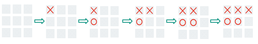
What is Quantum TiqTaqToe?

Evert van Nieuwenburg, the creator of Quantum TiqTaqToe whom I also collaborated with, goes in depth about how the game works here, but I will give a short rundown. The general idea is that there is now a split move, where you can put an ‘X’ in two different squares at once — a Schrödinger’s X, if you will. When the board has no more empty squares, the X randomly ‘collapses’ into one of the two squares with equal probability. The game ends when there are three real X’s or three real O’s in a row, just as in regular tic-tac-toe. Depending on the mode you are playing, you might also be able to entangle your X’s with your opponent’s O’s. You can get a better sense of all this by actually playing the game here.

My goal was to find out who wins when both players play optimally. For instance, in normal tic-tac-toe, it is well-known that the first X should go in the middle of the board, and if player O counters successfully, the game should end in a tie. Is the outcome of Quantum TiqTaqToe, too, predetermined to end in a tie if both players play optimally? And, if not, what is the best first move for player X? I sought to answer these questions through the power of computation.

The First Attempt

In the following section, I refer to a ‘game state’ as any unique arrangement of X’s and O’s on a board. The ‘empty game state’ simply means an empty board. ‘Traversing’ through a certain game state means that, at some point in the game, that game state occurs. So, for example, every game traverses through the empty game state, since every game starts with an empty board.

In order to solve the unsolved, one must first solve the solved. As such, my first attempt was to create an algorithm that would figure out the best move to play in regular tic-tac-toe. This first attempt was rather straightforward, and I will explain it here:

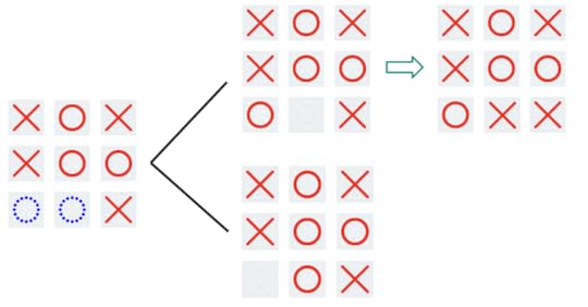
Essentially, I developed a model using what is known as “reinforcement learning” to determine the best next move given a certain game state. Here is how it works: To track which set of moves are best for player X and player O, respectively, every game state is assigned a value, initially 0. When a game ends, these values are updated to reflect who won. The more games are played, the better these values reflect the sequence of moves that X and O must make to win or tie. To train this model (machine learning parlance for the algorithm that updates the values/parameters mentioned above), I programmed the computer to play randomly chosen moves for X and O, until the game ended. If, say, player X won, then the value of every game state traversed was increased by 1 to indicate that X was favored. On the other hand, if player O won, then the value of every game state traversed was decreased by 1 to indicate that O was favored. Here is an example:

X wins!

Let’s say that this is the first iteration that the model is trained on. Then, the next time the model sees this game state,

it will recognize that X has an advantage. In the same vein, the model now also thinks that the empty game state is favorable towards X, since, in the one game that was played, when the empty game state was traversed, X won.

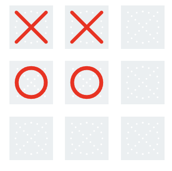
If we run these randomized games enough times (I ran ten million iterations), every move in every game state has most likely been made, which means that the model is able to give a meaningful evaluation for any game state. However, there is one major problem with this approach, in that the model only indicates who is favored when they make a random move, not when they make the best move. To illustrate this, let’s examine the following game state:

(O’s turn)

Here, player O has two options: they can win the game by putting their O on the bottom center square, or lose the game by putting it on the right center square. Any seasoned tic-tac-toe player would make the right move in this scenario, and win the game. However, since the model trains on random moves, it thinks that player O will win half the time and lose half the time. Thus, to the model, this game state is not favorable to either player, when in reality it is absolutely favored towards O. 

During my first meeting with Spiros and Evert, they pointed out this flaw in my model. Evert suggested that I study up on something called a minimax algorithm, which circumvents this flaw, and apply it to tic-tac-toe. This set me on the next step of my journey.

Enter Minimax

The content of this section takes inspiration from this article.

In the minimax algorithm, the two players are known as the ‘maximizer’ and the ‘minimizer’. In the case of tic-tac-toe, X would be the maximizer and O the minimizer. The maximizer’s goal is to maximize their score, while the minimizer’s goal is to minimize their score. In tic-tac-toe, the minimax algorithm is implemented so that a win by X is a score of +1, a win by O is a score of -1, and a tie is simply 0. So X, seeking to maximize their score, would want to win, which makes sense.

Now, if X wanted to maximize their score through some move, they would have to consider O’s move, who would try to minimize the score. But before O makes their move, they would have to consider X’s next move. This creates a sort of back-and-forth, recursive dynamic in the minimax algorithm. In order for either player to make the best move, they would have to go through all possible moves they can make, and all possible moves their opponent can make after that, and so on and so forth. Here is a relatively simple example of the minimax algorithm at work:

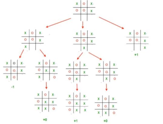
Let’s start from the top. X has three possible moves they can make, and evaluates each of them. 

In the leftmost branch, the result is either -1 or 0, but which is the real score? Well, we expect O to make their best move, and since they are trying to minimize the score, we expect them to choose the ‘-1’ case. So we can say that this move results in a score of -1. 

In the middle branch, the result is either 1 or 0, and, following the same reasoning as before, O chooses the move corresponding to the minimal score, resulting in a score of 0.

Finally, the last branch results in X winning, so the score is +1.

Now, X can finally choose their best move, and in the interest of maximizing the score, places their X on the bottom right square. Intuitively, this makes sense because it was the only move that wins the game for X outright.

Great, but what would a minimax algorithm look like in Quantum Tiqtaqtoe?

Enter Expecti-Minimax

Expectiminimax contains the same core idea as minimax, but something interesting happens when the game board collapses. The algorithm can’t know for sure what the board will look like after collapse, so all it can do is calculate an expected value of the result (hence the name). Let’s look at an example:

Here, collapse occurs, and one branch (top) results in a tie, while the other (bottom) results in O winning. Since a tie is equal to 0 and an O win is equal to -1, the algorithm treats the score as

Note: the sum is divided by two because both outcomes have a ½ probability of occurring.Solving the Game

Using the expecti-minimax algorithm, I effectively ‘solved’ the minimal and moderate versions of quantum tiqtaqtoe. However, even though the algorithm will always show the best move, the outcome from game to game might not be the same due to the inherent element of randomness. The most interesting of all my discoveries was probably the first move that the algorithm suggests for X, which I was able to make sense of both intuitively and logically. I challenge you all to find it! (Hint: it is the same for both the minimal and moderate versions.)

It turns out that when X plays optimally, they will always win the minimal version no matter what O plays. Meanwhile, in the moderate version, X will win most of the time, but not all the time. The probability distribution is as follows:

  (Another challenge: why are the denominators powers of two?)

Having satisfied my curiosity (for now), I’m looking forward to creating a new game of my own: 4 by 4 quantum tic-tac-toe. Currently, I am working on an algorithm that will give the best move, but since a 4×4 board is almost two times larger than a 3×3 board, the computational runtime of an expectiminimax algorithm would be far too large. As such, I am exploring the use of heuristics, which is sort of what the human mind uses to approach a game like tic-tac-toe. Because of this reliance on heuristics, there is no longer a guarantee that the algorithm will always make the best move, making this new adventure all the more mysterious and captivating. 

Crossing the quantum chasm: From NISQ to fault tolerance

On December 6, I gave a keynote address at the Q2B 2023 Conference in Silicon Valley. Here is a transcript of my remarks.

Toward quantum value

The theme of this year’s Q2B meeting is “The Roadmap to Quantum Value.” I interpret “quantum value” as meaning applications of quantum computing that have practical utility for end-users in business. So I’ll begin by reiterating a point I have made repeatedly in previous appearances at Q2B. As best we currently understand, the path to economic impact is the road through fault-tolerant quantum computing. And that poses daunting challenges for our field and for the quantum industry.

We are in the NISQ era. NISQ (rhymes with “risk’”) is an acronym meaning “Noisy Intermediate-Scale Quantum.” Here “intermediate-scale” conveys that current quantum computing platforms with of order 100 qubits are difficult to simulate by brute force using the most powerful currently existing supercomputers. “Noisy” reminds us that today’s quantum processors are not error-corrected, and noise is a serious limitation on their computational power. NISQ technology already has noteworthy scientific value. But as of now there is no proposed application of NISQ computing with commercial value for which quantum advantage has been demonstrated when compared to the best classical hardware running the best algorithms for solving the same problems. Furthermore, currently there are no persuasive theoretical arguments indicating that commercially viable applications will be found that do not use quantum error-correcting codes and fault-tolerant quantum computing.

A useful survey of quantum computing applications, over 300 pages long, recently appeared, providing rough estimates of end-to-end run times for various quantum algorithms. This is hardly the last word on the subject — new applications are continually proposed, and better implementations of existing algorithms continually arise. But it is a valuable snapshot of what we understand today, and it is sobering.

There can be quantum advantage in some applications of quantum computing to optimization, finance, and machine learning. But in this application area, the speedups are typically at best quadratic, meaning the quantum run time scales as the square root of the classical run time. So the advantage kicks in only for very large problem instances and deep circuits, which we won’t be able to execute without error correction.

Larger polynomial advantage and perhaps superpolynomial advantage is possible in applications to chemistry and materials science, but these may require at least hundreds of very well-protected logical qubits, and hundreds of millions of very high-fidelity logical gates, if not more. Quantum fault tolerance will be needed to run these applications, and fault tolerance has a hefty cost in both the number of physical qubits and the number of physical gates required. We should also bear in mind that the speed of logical gates is relevant, since the run time as measured by the wall clock will be an important determinant of the value of quantum algorithms.

Overcoming noise in quantum devices

Already in today’s quantum processors steps are taken to address limitations imposed by the noise — we use error mitigation methods like zero noise extrapolation or probabilistic error cancellation. These methods work effectively at extending the size of the circuits we can execute with useful fidelity. But the asymptotic cost scales exponentially with the size of the circuit, so error mitigation alone may not suffice to reach quantum value. Quantum error correction, on the other hand, scales much more favorably, like a power of a logarithm of the circuit size. But quantum error correction is not practical yet. To make use of it, we’ll need better two-qubit gate fidelities, many more physical qubits, robust systems to control those qubits, as well as the ability to perform fast and reliable mid-circuit measurements and qubit resets; all these are technically demanding goals.

To get a feel for the overhead cost of fault-tolerant quantum computing, consider the surface code — it’s presumed to be the best near-term prospect for achieving quantum error correction, because it has a high accuracy threshold and requires only geometrically local processing in two dimensions. Once the physical two-qubit error rate is below the threshold value of about 1%, the probability of a logical error per error correction cycle declines exponentially as we increase the code distance d:

Plogical = (0.1)(Pphysical/Pthreshold)(d+1)/2

where the number of physical qubits in the code block (which encodes a single protected qubit) is the distance squared.

Suppose we wish to execute a circuit with 1000 qubits and 100 million time steps. Then we want the probability of a logical error per cycle to be 10-11. Assuming the physical error rate is 10-3, better than what is currently achieved in multi-qubit devices, from this formula we infer that we need a code distance of 19, and hence 361 physical qubits to encode each logical qubit, and a comparable number of ancilla qubits for syndrome measurement — hence over 700 physical qubits per logical qubit, or a total of nearly a million physical qubits.  If the physical error rate improves to 10-4 someday, that cost is reduced, but we’ll still need hundreds of thousands of physical qubits if we rely on the surface code to protect this circuit.

Progress toward quantum error correction

The study of error correction is gathering momentum, and I’d like to highlight some recent experimental and theoretical progress. Specifically, I’ll remark on three promising directions, all with the potential to hasten the arrival of the fault-tolerant era: erasure conversion, biased noise, and more efficient quantum codes.

Erasure conversion

Error correction is more effective if we know when and where the errors occurred. To appreciate the idea, consider the case of a classical repetition code that protects against bit flips. If we don’t know which bits have errors we can decode successfully by majority voting, assuming that fewer than half the bits have errors. But if errors are heralded then we can decode successfully by just looking at any one of the undamaged bits. In quantum codes the details are more complicated but the same principle applies — we can recover more effectively if so-called erasure errors dominate; that is, if we know which qubits are damaged and in which time steps. “Erasure conversion” means fashioning a processor such that the dominant errors are erasure errors.

We can make use of this idea if the dominant errors exit the computational space of the qubit, so that an error can be detected without disturbing the coherence of undamaged qubits. One realization is with Alkaline earth Rydberg atoms in optical tweezers, where 0 is encoded as a low energy state, and 1 is a highly excited Rydberg state. The dominant error is the spontaneous decay of the 1 to a lower energy state. But if the atomic level structure and the encoding allow, 1 usually decays not to a 0, but rather to another state g. We can check whether the g state is occupied, to detect whether or not the error occurred, without disturbing a coherent superposition of 0 and 1.

Erasure conversion can also be arranged in superconducting devices, by using a so-called dual-rail encoding of the qubit in a pair of transmons or a pair of microwave resonators. With two resonators, for example, we can encode a qubit by placing a single photon in one resonator or the other. The dominant error is loss of the photon, causing either the 01 state or the 10 state to decay to 00. One can check whether the state is 00, detecting whether the error occurred, without disturbing a coherent superposition of 01 and 10.

Erasure detection has been successfully demonstrated in recent months, for both atomic (here and here) and superconducting (here and here) qubit encodings.

Biased noise

Another setting in which the effectiveness of quantum error correction can be enhanced is when the noise is highly biased. Quantum error correction is more difficult than classical error correction partly because more types of errors can occur — a qubit can flip in the standard basis, or it can flip in the complementary basis, what we call a phase error. In suitably designed quantum hardware the bit flips are highly suppressed, so we can concentrate the error-correcting power of the code on protecting against phase errors. For this scheme to work, it is important that phase errors occurring during the execution of a quantum gate do not propagate to become bit-flip errors. And it was realized just a few years ago that such bias-preserving gates are possible for qubits encoded in continuous variable systems like microwave resonators.

Specifically, we may consider a cat code, in which the encoded 0 and encoded 1 are coherent states, well separated in phase space. Then bit flips are exponentially suppressed as the mean photon number in the resonator increases. The main source of error, then, is photon loss from the resonator, which induces a phase error for the cat qubit, with an error rate that increases only linearly with photon number. We can then strike a balance, choosing a photon number in the resonator large enough to provide physical protection against bit flips, and then use a classical code like the repetition code to build a logical qubit well protected against phase flips as well.

Work on such repetition cat codes is ongoing (see here, here, and here), and we can expect to hear about progress in that direction in the coming months.

More efficient codes

Another exciting development has been the recent discovery of quantum codes that are far more efficient than the surface code. These include constant-rate codes, in which the number of protected qubits scales linearly with the number of physical qubits in the code block, in contrast to the surface code, which protects just a single logical qubit per block. Furthermore, such codes can have constant relative distance, meaning that the distance of the code, a rough measure of how many errors can be corrected, scales linearly with the block size rather than the square root scaling attained by the surface code.

These new high-rate codes can have a relatively high accuracy threshold, can be efficiently decoded, and schemes for executing fault-tolerant logical gates are currently under development.

A drawback of the high-rate codes is that, to extract error syndromes, geometrically local processing in two dimensions is not sufficient — long-range operations are needed. Nonlocality can be achieved through movement of qubits in neutral atom tweezer arrays or ion traps, or one can use the native long-range coupling in an ion trap processor. Long-range coupling is more challenging to achieve in superconducting processors, but should be possible.

An example with potential near-term relevance is a recently discovered code with distance 12 and 144 physical qubits. In contrast to the surface code with similar distance and length which encodes just a single logical qubit, this code protects 12 logical qubits, a significant improvement in encoding efficiency.

The quest for practical quantum error corrections offers numerous examples like these of co-design. Quantum error correction schemes are adapted to the features of the hardware, and ideas about quantum error correction guide the realization of new hardware capabilities. This fruitful interplay will surely continue.

An exciting time for Rydberg atom arrays

In this year’s hardware news, now is a particularly exciting time for platforms based on Rydberg atoms trapped in optical tweezer arrays. We can anticipate that Rydberg platforms will lead the progress in quantum error correction for at least the next few years, if two-qubit gate fidelities continue to improve. Thousands of qubits can be controlled, and geometrically nonlocal operations can be achieved by reconfiguring the atomic positions. Further improvement in error correction performance might be possible by means of erasure conversion. Significant progress in error correction using Rydberg platforms is reported in a paper published today.

But there are caveats. So far, repeatable error syndrome measurement has not been demonstrated. For that purpose, continuous loading of fresh atoms needs to be developed. And both the readout and atomic movement are relatively slow, which limits the clock speed.

Movability of atomic qubits will be highly enabling in the short run. But in the longer run, movement imposes serious limitations on clock speed unless much faster movement can be achieved. As things currently stand, one can’t rapidly accelerate an atom without shaking it loose from an optical tweezer, or rapidly accelerate an ion without heating its motional state substantially. To attain practical quantum computing using Rydberg arrays, or ion traps, we’ll eventually need to make the clock speed much faster.

Cosmic rays!

To be fair, other platforms face serious threats as well. One is the vulnerability of superconducting circuits to ionizing radiation. Cosmic ray muons for example will occasionally deposit a large amount of energy in a superconducting circuit, creating many phonons which in turn break Cooper pairs and induce qubit errors in a large region of the chip, potentially overwhelming the error-correcting power of the quantum code. What can we do? We might go deep underground to reduce the muon flux, but that’s expensive and inconvenient. We could add an additional layer of coding to protect against an event that wipes out an entire surface code block; that would increase the overhead cost of error correction. Or maybe modifications to the hardware can strengthen robustness against ionizing radiation, but it is not clear how to do that.

Outlook

Our field and the quantum industry continue to face a pressing question: How will we scale up to quantum computing systems that can solve hard problems? The honest answer is: We don’t know yet. All proposed hardware platforms need to overcome serious challenges. Whatever technologies may seem to be in the lead over, say, the next 10 years might not be the best long-term solution. For that reason, it remains essential at this stage to develop a broad array of hardware platforms in parallel.

Today’s NISQ technology is already scientifically useful, and that scientific value will continue to rise as processors advance. The path to business value is longer, and progress will be gradual. Above all, we have good reason to believe that to attain quantum value, to realize the grand aspirations that we all share for quantum computing, we must follow the road to fault tolerance. That awareness should inform our thinking, our strategy, and our investments now and in the years ahead.

Crossing the quantum chasm (image generated using Midjourney)

The power of awe

Mid-afternoon, one Saturday late in September, I forgot where I was. I forgot that I was visiting Seattle for the second time; I forgot that I’d just finished co-organizing a workshop partially about nuclear physics for the first time. I’d arrived at a crowded doorway in the Chihuly Garden and Glass museum, and a froth of blue was towering above the onlookers in front of me. Glass tentacles, ranging from ultramarine through turquoise to clear, extended from the froth. Golden conch shells, starfish, and mollusks rode the waves below. The vision drove everything else from my mind for an instant.

Much had been weighing on my mind that week. The previous day had marked the end of a workshop hosted by the Inqubator for Quantum Simulation (IQuS, pronounced eye-KWISS) at the University of Washington. I’d co-organized the workshop with IQuS member Niklas Mueller, NIST physicist Alexey Gorshkov, and nuclear theorist Raju Venugopalanan (although Niklas deserves most of the credit). We’d entitled the workshop “Thermalization, from Cold Atoms to Hot Quantum Chromodynamics.” Quantum chromodynamics describes the strong force that binds together a nucleus’s constituents, so I call the workshop “Journey to the Center of the Atom” to myself. 

We aimed to unite researchers studying thermal properties of quantum many-body systems from disparate perspectives. Theorists and experimentalists came; and quantum information scientists and nuclear physicists; and quantum thermodynamicists and many-body physicists; and atomic, molecular, and optical physicists. Everyone cared about entanglement, equilibration, and what else happens when many quantum particles crowd together and interact. 

We quantum physicists crowded together and interacted from morning till evening. We presented findings to each other, questioned each other, coagulated in the hallways, drank tea together, and cobbled together possible projects. The week electrified us like a chilly ocean wave but also wearied me like an undertow. Other work called for attention, and I’d be presenting four more talks at four more workshops and campus visits over the next three weeks. The day after the workshop, I worked in my hotel half the morning and then locked away my laptop. I needed refreshment, and little refreshes like art.

Strongly interacting physicists

Chihuly Garden and Glass, in downtown Seattle, succeeded beyond my dreams: the museum drew me into somebody else’s dreams. Dale Chihuly grew up in Washington state during the mid-twentieth century. He studied interior design and sculpture before winning a Fulbright Fellowship to learn glass-blowing techniques in Murano, Italy. After that, Chihuly transformed the world. I’ve encountered glass sculptures of his in Pittsburgh; Florida; Boston; Jerusalem; Washington, DC; and now Seattle—and his reach dwarfs my travels. 

Chihuly chandelier at the Renwick Gallery in Washington, DC

After the first few encounters, I began recognizing sculptures as Chihuly’s before checking their name plates. Every work by his team reflects his style. Tentacles, bulbs, gourds, spheres, and bowls evidence what I never expected glass to do but what, having now seen it, I’m glad it does.

This sentiment struck home a couple of galleries beyond the Seaforms. The exhibit Mille Fiori drew inspiration from the garden cultivated by Chihuly’s mother. The name means A Thousand Flowers, although I spied fewer flowers than what resembled grass, toadstools, and palm fronds. Visitors feel like grasshoppers amongst the red, green, and purple stalks that dwarfed some of us. The narrator of Jules Vernes’s Journey to the Center of the Earth must have felt similarly, encountering mastodons and dinosaurs underground. I encircled the garden before registering how much my mind had lightened. Responsibilities and cares felt miles away—or, to a grasshopper, backyards away. Wonder does wonders.

Mille Fiori

Near the end of the path around the museum, a theater plays documentaries about Chihuly’s projects. The documentaries include interviews with the artist, and several quotes reminded me of the science I’d been trained to seek out: “I really wanted to take glass to its glorious height,” Chihuly said, “you know, really make something special.” “Things—pieces got bigger, pieces got taller, pieces got wider.” He felt driven to push art forms as large as the glass would permit his team. Similarly, my PhD advisor John Preskill encouraged me to “think big.” What physics is worth doing—what would create an impact?

How did a boy from Tacoma, Washington impact not only fellow blown-glass artists—not only artists—not only an exhibition here and there in his home country—but experiences across the globe, including that of a physicist one weekend in September?

One idea from the IQuS workshop caught my eye. Some particle colliders accelerate heavy ions to high energies and then smash the ions together. Examples include lead and gold ions studied at CERN in Geneva. After a collision, the matter expands and cools. Nuclear physicists don’t understand how the matter cools; models predict cooling times longer than those observed. This mismatch has persisted across decades of experiments. The post-collision matter evades attempts at computer simulation; it’s literally a hot mess. Can recent advances in many-body physics help?

The exhibit Persian Ceiling at Chihuly Garden and Glass. Doesn’t it look like it could double as an artist’s rendering of a heavy-ion collision?

Martin Savage, the director of IQuS, hopes so. He hopes that IQuS will impact nuclear physics across the globe. Every university and its uncle boasts a quantum institute nowadays, but IQuS seems to me to have carved out a niche for itself. IQuS has grown up in the bosom of the Institute for Nuclear Theory at the University of Washington, which has guided nuclear theory for decades. IQuS is smashing that history together with the future of quantum simulators. IQuS doesn’t strike me as just another glass bowl in the kitchen of quantum science. A bowl worthy of Chihuly? I don’t know, but I’d like to hope so.

I left Chihuly Garden and Glass with respect for the past week and energy for the week ahead. Whether you find it in physics or in glass or in both—or in plunging into a dormant Icelandic volcano in search of the Earth’s core—I recommend the occasional dose of awe.

Participants in the final week of the workshop

With thanks to Martin Savage, IQuS, and the University of Washington for their hospitality.

Astrobiology meets quantum computation?

The origin of life appears to share little with quantum computation, apart from the difficulty of achieving it and its potential for clickbait. Yet similar notions of complexity have recently garnered attention in both fields. Each topic’s researchers expect only special systems to generate high values of such complexity, or complexity at high rates: organisms, in one community, and quantum computers (and perhaps black holes), in the other. 

Each community appears fairly unaware of its counterpart. This article is intended to introduce the two. Below, I review assembly theory from origin-of-life studies, followed by quantum complexity. I’ll then compare and contrast the two concepts. Finally, I’ll suggest that origin-of-life scientists can quantize assembly theory using quantum complexity. The idea is a bit crazy, but, well, so what?

Assembly theory in origin-of-life studies

Imagine discovering evidence of extraterrestrial life. How could you tell that you’d found it? You’d have detected a bunch of matter—a bunch of particles, perhaps molecules. What about those particles could evidence life?

This question motivated Sara Imari Walker and Lee Cronin to develop assembly theory. (Most of my assembly-theory knowledge comes from Sara, about whom I wrote this blog post years ago and with whom I share a mentor.) Assembly theory governs physical objects, from proteins to self-driving cars. 

Imagine assembling a protein from its constituent atoms. First, you’d bind two atoms together. Then, you might bind another two atoms together. Eventually, you’d bind two pairs together. Your sequence of steps would form an algorithm for assembling the protein. Many algorithms can generate the same protein. One algorithm has the least number of steps. That number is called the protein’s assembly number.

Different natural processes tend to create objects that have different assembly numbers. Stars form low-assembly-number objects by fusing two hydrogen atoms together into helium. Similarly, random processes have high probabilities of forming low-assembly-number objects. For example, geological upheavals can bring a shard of iron near a lodestone. The iron will stick to the magnetized stone, forming a two-component object.

My laptop has an enormous assembly number. Why can such an object exist? Because of information, Sara and Lee emphasize. Human beings amassed information about materials science, Boolean logic, the principles of engineering, and more. That information—which exists only because organisms exists—helped engender my laptop.

If any object has a high enough assembly number, Sara and Lee posit, that object evidences life. Absent life, natural processes have too low a probability of randomly throwing together molecules into the shape of a computer. How high is “high enough”? Approximately fifteen, experiments by Lee’s group suggest. (Why do those experiments point to the number fifteen? Sara’s group is working on a theory for predicting the number.)

In summary, assembly number quantifies complexity in origin-of-life studies, according to Sara and Lee. The researchers propose that only living beings create high-assembly-number objects.

Quantum complexity in quantum computation

Quantum complexity defines a stage in the equilibration of many-particle quantum systems. Consider a clump of quantum particles isolated from its environment. The clump will be in a pure quantum state at a time . The particles will interact, evolving the clump’s state as a function  . 

Quantum many-body equilibration is more complicated than the equilibration undergone by your afternoon pick-me-up as it cools.

The interactions will equilibrate the clump internally. One stage of equilibration centers on local observables . They’ll come to have expectation values approximately equal to thermal expectation values , for a thermal state  of the clump. During another stage of equilibration, the particles correlate through many-body entanglement. 

The longest known stage centers on the quantum complexity of . The quantum complexity is the minimal number of basic operations needed to prepare from a simple initial state. We can define “basic operations” in many ways. Examples include quantum logic gates that act on two particles. Another example is an evolution for one time step under a Hamiltonian that couples together at most particles, for some independent of . Similarly, we can define “a simple initial state” in many ways. We could count as simple only the -fold tensor product of our favorite single-particle state . Or we could call any -fold tensor product simple, or any state that contains at-most-two-body entanglement, and so on. These choices don’t affect the quantum complexity’s qualitative behavior, according to string theorists Adam Brown and Lenny Susskind.

How quickly can the quantum complexity of grow? Fast growth stems from many-body interactions, long-range interactions, and random coherent evolutions. (Random unitary circuits exemplify random coherent evolutions: each gate is chosen according to the Haar measure, which we can view roughly as uniformly random.) At most, quantum complexity can grow linearly in time. Random unitary circuits achieve this rate. Black holes may; they scramble information quickly. The greatest possible complexity of any -particle state scales exponentially in , according to a counting argument. 

A highly complex state looks simple from one perspective and complicated from another. Human scientists can easily measure only local observables . Such observables’ expectation values   tend to look thermal in highly complex states, , as implied above. The thermal state has the greatest von Neumann entropy, , of any quantum state that obeys the same linear constraints as (such as having the same energy expectation value). Probed through simple, local observables , highly complex states look highly entropic—highly random—similarly to a flipped coin.

Yet complex states differ from flipped coins significantly, as revealed by subtler analyses. An example underlies the quantum-supremacy experiment published by Google’s quantum-computing group in 2018. Experimentalists initialized 53 qubits (quantum two-level systems) in a tensor product. The state underwent many gates, which prepared a highly complex state. Then, the experimentalists measured the -component of each qubit’s spin, randomly obtaining a -1 or a 1. One trial yielded a 53-bit string. The experimentalists repeated this process many times, using the same gates in each trial. From all the trials’ bit strings, the group inferred the probability of obtaining a given string in the next trial. The distribution resembles the uniformly random distribution…but differs from it subtly, as revealed by a cross-entropy analysis. Classical computers can’t easily generate ; hence the Google group’s claiming to have achieved quantum supremacy/advantage. Quantum complexity differs from simple randomness, that difference is difficult to detect, and the difference can evidence quantum computers’ power.

A fridge that holds one of Google’s quantum computers.

Comparison and contrast

Assembly number and quantum complexity resemble each other as follows:

Each function quantifies the fewest basic operations needed to prepare something.Only special systems (organisms) can generate high assembly numbers, according to Sara and Lee. Similarly, only special systems (such as quantum computers and perhaps black holes) can generate high complexity quickly, quantum physicists expect.Assembly number may distinguish products of life from products of abiotic systems. Similarly, quantum complexity helps distinguish quantum computers’ computational power from classical computers’.High-assembly-number objects are highly structured (think of my laptop). Similarly, high-complexity quantum states are highly structured in the sense of having much many-body entanglement.Organisms generate high assembly numbers, using information. Similarly, using information, organisms have created quantum computers, which can generate quantum complexity quickly.

Assembly number and quantum complexity differ as follows:

Classical objects have assembly numbers, whereas quantum states have quantum complexities.In the absence of life, random natural processes have low probabilities of producing high-assembly-number objects. That is, randomness appears to keep assembly numbers low. In contrast, randomness can help quantum complexity grow quickly.Highly complex quantum states look very random, according to simple, local probes. High-assembly-number objects do not.Only organisms generate high assembly numbers, according to Sara and Lee. In contrast, abiotic black holes may generate quantum complexity quickly.

Another feature shared by assembly-number studies and quantum computation merits its own paragraph: the importance of robustness. Suppose that multiple copies of a high-assembly-number (or moderate-assembly-number) object exist. Not only does my laptop exist, for example, but so do many other laptops. To Sara, such multiplicity signals the existence of some stable mechanism for creating that object. The multiplicity may provide extra evidence for life (including life that’s discovered manufacturing), as opposed to an unlikely sequence of random forces. Similarly, quantum computing—the preparation of highly complex states—requires stability. Decoherence threatens quantum states, necessitating quantum error correction. Quantum error correction differs from Sara’s stable production mechanism, but both evidence the importance of robustness to their respective fields.

A modest proposal

One can generalize assembly number to quantum states, using quantum complexity. Imagine finding a clump of atoms while searching for extraterrestrial life. The atoms need not have formed molecules, so the clump can have a low classical assembly number. However, the clump can be in a highly complex quantum state. We could detect the state’s complexity only (as far as I know) using many copies of the state, so imagine finding many clumps of atoms. Preparing highly complex quantum states requires special conditions, such as a quantum computer. The clump might therefore evidence organisms who’ve discovered quantum physics. Using quantum complexity, one might extend the assembly number to identify quantum states that may evidence life. However, quantum complexity, or a high rate of complexity generation, alone may not evidence life—for example, if achievable by black holes. Fortunately, a black hole seems unlikely to generate many identical copies of a highly complex quantum state. So we seem to have a low probability of mistakenly attributing a highly complex quantum state, sourced by a black hole, to organisms (atop our low probability of detecting any complex quantum state prepared by anyone other than us).

Would I expect a quantum assembly number to greatly improve humanity’s search for extraterrestrial life? I’m no astrobiology expert (NASA videos notwithstanding), but I’d expect probably not. Still, astrobiology requires chemistry, which requires quantum physics. Quantum complexity seems likely to find applications in the assembly-number sphere. Besides, doesn’t juxtaposing the search for extraterrestrial life and the understanding of life’s origins with quantum computing sound like fun? And a sense of fun distinguishes certain living beings from inanimate matter about as straightforwardly as assembly number does.

With thanks to Jim Al-Khalili, Paul Davies, the From Physics to Life collaboration, and UCLA for hosting me at the workshop that spurred this article.

May I have this dance?

This July, I came upon a museum called the Haus der Musik in one of Vienna’s former palaces. The museum contains a room dedicated to Johann Strauss II, king of the waltz. The room, dimly lit, resembles a twilit gazebo. I could almost believe that a hidden orchestra was playing the rendition of “The Blue Danube” that filled the room. Glass cases displayed dance cards and accessories that dancers would bring to a nineteenth-century ball.

A ball. Who hasn’t read about one in a novel or seen one in a film? A throng of youngsters and their chaperones, rustling in silk. The glint of candles, the vigor of movement, the thrill of interaction, the anxiety of establishing one’s place in society.

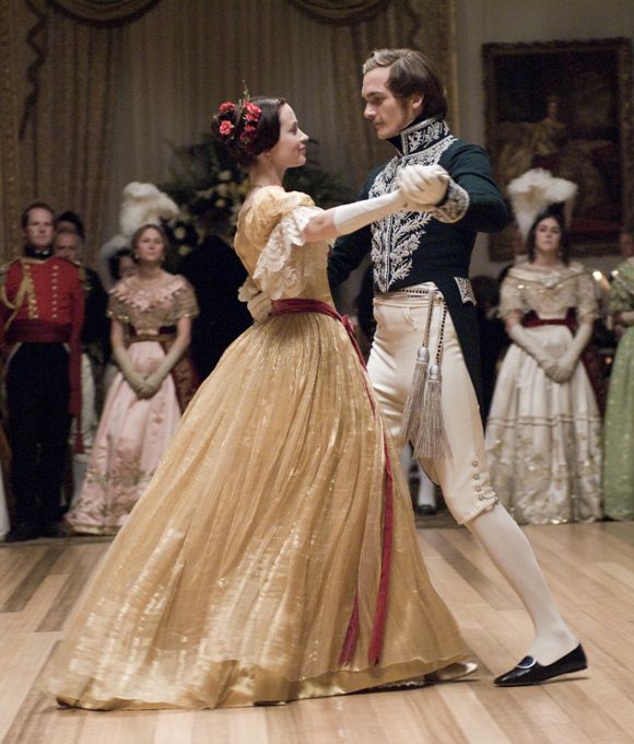Victoria and Albert at a ball in the film The Young Victoria

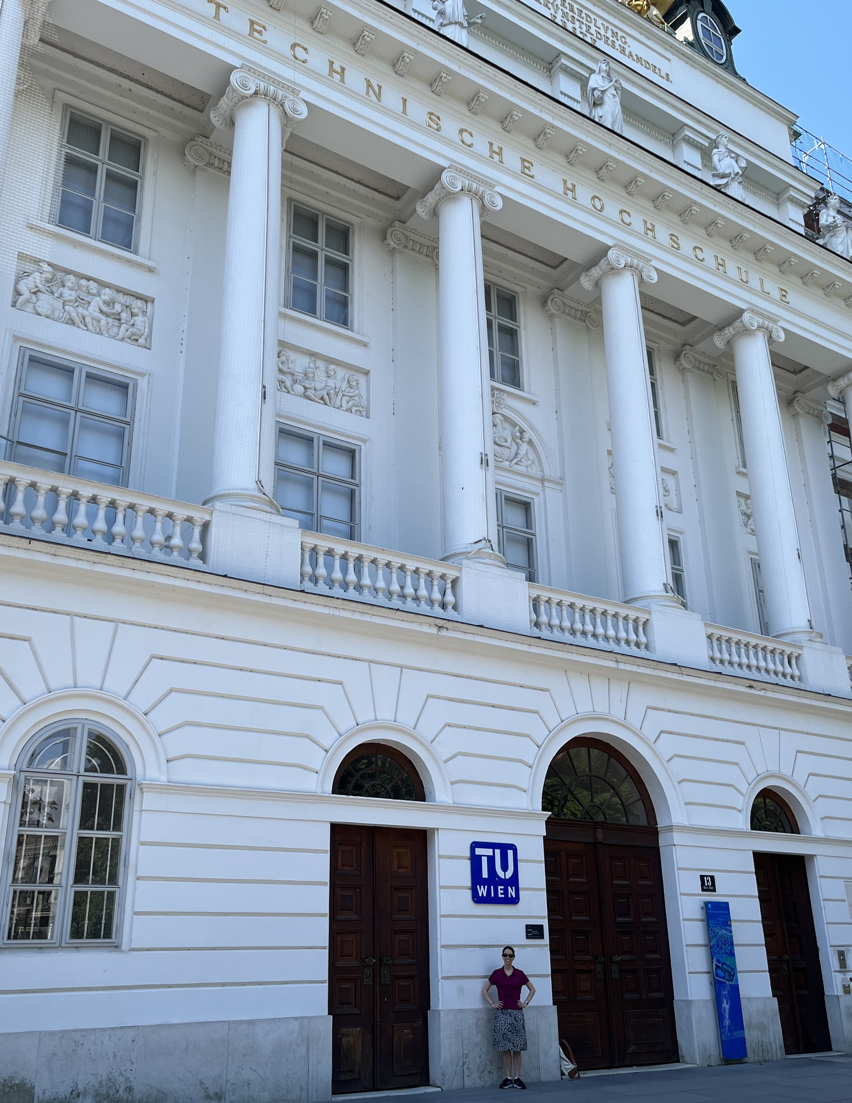
Another throng gathered a short walk from the Haus der Musik this summer. The Vienna University of Technology hosted the conference Quantum Thermodynamics (QTD) in the heart of the city. Don’t tell the other annual conferences, but QTD is my favorite. It spotlights the breed of quantum thermodynamics that’s surged throughout the past decade—the breed saturated with quantum information theory. I began attending QTD as a PhD student, and the conference shifts from city to city from year to year. I reveled in returning in person for the first time since the pandemic began.

Yet this QTD felt different. First, instead of being a PhD student, I brought a PhD student of my own. Second, granted, I enjoyed catching up with colleagues-cum-friends as much as ever. I especially relished seeing the “classmates” who belonged to my academic generation. Yet we were now congratulating each other on having founded research groups, and we were commiserating about the workload of primary investigators. 

Third, I found myself a panelist in the annual discussion traditionally called “Quo vadis, quantum thermodynamics?” The panel presented bird’s-eye views on quantum thermodynamics, analyzing trends and opining on the direction our field was taking (or should take).1 Fourth, at the end of the conference, almost the last sentence spoken into any microphone was “See you in Maryland next year.” Colleagues and I will host QTD 2024.

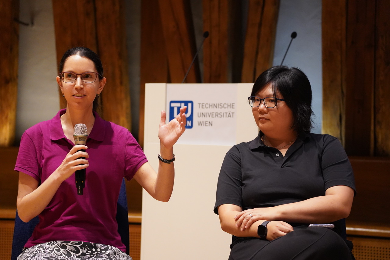
One of my dearest quantum-thermodynamic “classmates,” Nelly Ng, participated in the panel discussion, too. We met as students (see these two blog posts), and she’s now an assistant professor at Nanyang Technological University. Photo credit: Jakub Czartowski.

The day after QTD ended, I boarded an Austrian Airlines flight. Waltzes composed by Strauss played over the loudspeakers. They flipped a switch in my mind: I’d come of age, I thought. I’d attended QTD 2017 as a debutante, presenting my first invited talk at the conference series. I’d danced through QTD 2018 in Santa Barbara, as well as the online iterations held during the pandemic. I’d reveled in the vigor of scientific argumentation, the thrill of learning, the glint of slides shining on projector screens (not really). Now, I was beginning to shoulder responsibilities like a ballgown-wearing chaperone.

As I came of age, so did QTD. The conference series budded around the time I started grad school and embarked upon quantum-thermodynamics research. In 2017, approximately 80 participants attended QTD. This year, 250 people registered to attend in person, and others attended online. Two hundred fifty! Quantum thermodynamics scarcely existed as a field of research fifteen years ago.

I’ve heard that organizers of another annual conference, Quantum Information Processing (QIP), reacted similarly to a 250-person registration list some years ago. Aram Harrow, a professor and quantum information theorist at MIT, has shared stories about co-organizing the first QIPs. As a PhD student, he’d sat in his advisor’s office, taking notes, while the local quantum-information theorists chose submissions to highlight. Nowadays, a small army of reviewers and subreviewers processes the hordes of submissions. And, from what I heard about this year’s attendance, you almost might as well navigate a Disney theme park on a holiday as the QIP crowd. 

Will QTD continue to grow like QIP? Would such growth strengthen or fracture the community? Perhaps we’ll discuss those questions at a “Quo vadis?” session in Maryland next year. But I, at least, hope to continue always to grow—and to dance.2

Ludwig Boltzmann, a granddaddy of thermodynamics, worked in Vienna. I’ve waited for years to make a pilgrimage.

1My opinion: Now that quantum thermodynamics has showered us with fundamental insights, we should apply it in practical applications. How? Collaborators and I suggest one path here.

2I confess to having danced the waltz step (gleaned during my 14 years of ballet training) around that Strauss room in the Haus der Musik. I didn’t waltz around the conference auditorium, though.

Can Thermodynamics Resolve the Measurement Problem?

At the recent Quantum Thermodynamics conference in Vienna (coming next year to the University of Maryland!), during an expert panel Q&A session, one member of the audience asked “can quantum thermodynamics address foundational problems in quantum theory?”

That stuck with me, because that’s exactly what my research is about. So naturally, I’d say the answer is yes! In fact, here in the group of Marcus Huber at the Technical University of Vienna, we think thermodynamics may have something to say about the biggest quantum foundations problem of all: the measurement problem.

It’s sort of the iconic mystery of quantum mechanics: we know that an electron can be in two places at once – in a ‘superposition’ – but when we measure it, it’s only ever seen to be in one place, picked seemingly at random from the two possibilities. We say the state has ‘collapsed’.

What’s going on here? Thanks to Bell’s legendary theorem, we know that the answer can’t just be that it was always actually in one place and we just didn’t know which option it was – it really was in two places at once until it was measured1. But also, we don’t see this effect for sufficiently large objects. So how can this ‘two-places-at-once’ thing happen at all, and why does it stop happening once an object gets big enough?

Here, we already see hints that thermodynamics is involved, because even classical thermodynamics says that big systems behave differently from small ones. And interestingly, thermodynamics also hints that the narrative so far can’t be right. Because when taken at face value, the ‘collapse’ model of measurement breaks all three laws of thermodynamics.

Imagine an electron in a superposition of two energy levels: a combination of being in its ground state and first excited state. If we measure it and it ‘collapses’ to being only in the ground state, then its energy has decreased: it went from having some average of the ground and excited energies to just having the ground energy. The first law of thermodynamics says (crudely) that energy is conserved, but the loss of energy is unaccounted for here.

Next, the second law says that entropy always increases. One form of entropy represents your lack of information about a system’s state. Before the measurement, the system was in one of two possible states, but afterwards it was in only one state. So speaking very broadly, our uncertainty about its state, and hence the entropy, is reduced. (The third law is problematic here, too.)

There’s a clear explanation here: while the system on its own decreases its entropy and doesn’t conserve energy, in order to measure something, we must couple the system to a measuring device. That device’s energy and entropy changes must account for the system’s changes.

This is the spirit of our measurement model2. We explicitly include the detector as a quantum object in the record-keeping of energy and information flow. In fact, we also include the entire environment surrounding both system and device – all the lab’s stray air molecules, photons, etc. Then the idea is to describe a measurement process as propagating a record of a quantum system’s state into the surroundings without collapsing it.

A schematic representation of a system spreading information into an environment (from Schwarzhans et al., with permission)

But talking about quantum systems interacting with their environments is nothing new. The “decoherence” model from the 70s, which our work builds on, says quantum objects become less quantum when buffeted by a larger environment.

The problem, though, is that decoherence describes how information is lost into an environment, and so usually the environment’s dynamics aren’t explicitly calculated: this is called an open-system approach. By contrast, in the closed-system approach we use, you model the dynamics of the environment too, keeping track of all information. This is useful because conventional collapse dynamics seems to destroy information, but every other fundamental law of physics seems to say that information can’t be destroyed.

This all allows us to track how information flows from system to surroundings, using the “Quantum Darwinism” (QD) model of W.H. Żurek. Whereas decoherence describes how environments affect systems, QD describes how quantum systems impact their environments by spreading information into them. The QD model says that the most ‘classical’ information – the kind most consistent with classical notions of ‘being in one place’, etc. – is the sort most likely to ‘survive’ the decoherence process.

QD then further asserts that this is the information that’s most likely to be copied into the environment. If you look at some of a system’s surroundings, this is what you’d most likely see. (The ‘Darwinism’ name is because certain states are ‘selected for’ and ‘replicate’3.)

So we have a description of what we want the post-measurement state to look like: a decohered system, with its information redundantly copied into its surrounding environment. The last piece of the puzzle, then, is to ask how a measurement can create this state. Here, we finally get to the dynamics part of the thermodynamics, and introduce equilibration.

Earlier we said that even if the system’s entropy decreases, the detector’s entropy (or more broadly the environment’s) should go up to compensate. Well, equilibration maximizes entropy. In particular, equilibration describes how a system tends towards a particular ‘equilibrium’ state, because the system can always increase its entropy by getting closer to it.

It’s usually said that systems equilibrate if put in contact with an external environment (e.g. a can of beer cooling in a fridge), but we’re actually interested in a different type of equilibration called equilibration on average. There, we’re asking for the state that a system stays roughly close to, on average, over long enough times, with no outside contact. That means it never actually decoheres, it just looks like it does for certain observables. (This actually implies that nothing ever actually decoheres, since open systems are only an approximation you make when you don’t want to track all of the environment.)

Equilibration is the key to the model. In fact, we call our idea the Measurement-Equilibration Hypothesis (MEH): we’re asserting that measurement is an equilibration process. Which makes the final question: what does all this mean for the measurement problem?

In the MEH framework, when someone ‘measures’ a quantum system, they allow some measuring device, plus a chaotic surrounding environment, to interact with it. The quantum system then equilibrates ‘on average’ with the environment, and spreads information about its classical states into the surroundings. Since you are a macroscopically large human, any measurement you do will induce this sort of equilibration to happen, meaning you will only ever have access to the classical information in the environment, and never see superpositions. But no collapse is necessary, and no information is lost: rather some information is only much more difficult to access in all the environment noise, as happens all the time in the classical world.

It’s tempting to ask what ‘happens’ to the outcomes we don’t see, and how nature ‘decides’ which outcome to show to us. Those are great questions, but in our view, they’re best left to philosophers4. For the question we care about: why measurements look like a ‘collapse’, we’re just getting started with our Measurement-Equilibration Hypothesis – there’s still lots to do in our explorations of it. We think the answers we’ll uncover in doing so will form an exciting step forward in our understanding of the weird and wonderful quantum world.

Members of the MEH team at a kick-off meeting for the project in Vienna in February 2023. Left to right: Alessandro Candeloro, Marcus Huber, Emanuel Schwarzhans, Tom Rivlin, Sophie Engineer, Veronika Baumann, Nicolai Friis, Felix C. Binder, Mehul Malik, Maximilian P.E. Lock, Pharnam Bakhshinezhad

Acknowledgements: Big thanks to the rest of the MEH team for all the help and support, in particular Dr. Emanuel Schwarzhans and Dr. Lock for reading over this piece!)

Here are a few choice references (by no means meant to be comprehensive!)

Quantum Thermodynamics (QTD) Conference 2023: https://qtd2023.conf.tuwien.ac.at/
QTD 2024: https://qtd-hub.umd.edu/event/qtd-conference-2024/
Bell’s Theorem: https://plato.stanford.edu/entries/bell-theorem/
The first MEH paper: https://arxiv.org/abs/2302.11253
A review of decoherence: https://journals.aps.org/rmp/abstract/10.1103/RevModPhys.75.715
Quantum Darwinism: https://www.nature.com/articles/nphys1202
Measurements violate the 3rd law: https://quantum-journal.org/papers/q-2020-01-13-222/
More on the 3rd and QM: https://journals.aps.org/prxquantum/abstract/10.1103/PRXQuantum.4.010332
Equilibration on average: https://iopscience.iop.org/article/10.1088/0034-4885/79/5/056001/meta
Objectivity: https://journals.aps.org/pra/abstract/10.1103/PhysRevA.91.032122

There is a perfectly valid alternative with other weird implications: that it was always just in one place, but the world is intrinsically non-local. Most physicists prefer to save locality over realism, though. ︎First proposed in this paper by Schwarzhans, Binder, Huber, and Lock: https://arxiv.org/abs/2302.11253 ︎In my opinion… it’s a brilliant theory with a terrible name! Sure, there’s something akin to ‘selection pressure’ and ‘reproduction’, but there aren’t really any notions of mutation, adaptation, fitness, generations… Alas, the name has stuck. ︎I actually love thinking about this question, and the interpretations of quantum mechanics more broadly, but it’s fairly orthogonal to the day-to-day research on this model. ︎

The Book of Mark, Chapter 2

Late in the summer of 2021, I visited a physics paradise in a physical paradise: the Kavli Institute for Theoretical Physics (KITP). The KITP sits at the edge of the University of California, Santa Barbara like a bougainvillea bush at the edge of a yard. I was eating lunch outside the KITP one afternoon, across the street from the beach. PhD student Arman Babakhani, whom a colleague had just introduced me to, had joined me.

The KITP’s Kohn Hall

What physics was I working on nowadays? Arman wanted to know.

Thermodynamic exchanges. 

The world consists of physical systems exchanging quantities with other systems. When a rose blooms outside the Santa Barbara mission, it exchanges pollen with the surrounding air. The total amount of pollen across the rose-and-air whole remains constant, so we call the amount a conserved quantity. Quantum physicists usually analyze conservation of particles, energy, and magnetization. But quantum systems can conserve quantities that participate in uncertainty relations. Such quantities are called incompatible, because you can’t measure them simultaneously. The -, -, and -components of a qubit’s spin are incompatible.

The Santa Barbara mission… …and its roses

Exchanging and conserving incompatible quantities, systems can violate thermodynamic expectations. If one system is much larger than the other, we expect the smaller system to thermalize; yet incompatibility invalidates derivations of the thermal state’s form. Incompatibility reduces the thermodynamic entropy produced by exchanges. And incompatibility can raise the average amount entanglement in the pair of systems—the total system.

If the total system conserves incompatible quantities, what happens to the eigenstate thermalization hypothesis (ETH)? Last month’s blog post overviewed the ETH, a framework for understanding how quantum many-particle systems thermalize internally. That post labeled Mark Srednicki, a professor at the KITP, a high priest of the ETH. I want, I told Arman, to ask Mark what happens when you combine the ETH with incompatible conserved quantities.

I’ll do it, Arman said.

Soon after, I found myself in the fishbowl. High up in the KITP, a room filled with cushy seats overlooks the ocean. The circular windows lend the room its nickname. Arrayed on the armchairs and couches were Mark, Arman, Mark’s PhD student Fernando Iniguez, and Mark’s recent PhD student Chaitanya Murthy. The conversation went like this:

Mark was frustrated about not being able to answer the question. I was delighted to have stumped him. Over the next several weeks, the group continued meeting, and we emailed out notes for everyone to criticize. I particulary enjoyed watching Mark and Chaitanya interact. They’d grown so intellectually close throughout Chaitanya’s PhD studies, they reminded me of an old married couple. One of them had to express only half an idea for the other to realize what he’d meant and to continue the thread. Neither had any qualms with challenging the other, yet they trusted each other’s judgment.1

In vintage KITP fashion, we’d nearly completed a project by the time Chaitanya and I left Santa Barbara. Physical Review Letters published our paper this year, and I’m as proud of it as a gardener of the first buds from her garden. Here’s what we found.

Southern California spoiled me for roses.

Incompatible conserved quantities conflict with the ETH and the ETH’s prediction of internal thermalization. Why? For three reasons. First, when inferring thermalization from the ETH, we assume that the Hamiltonian lacks degeneracies (that no energy equals any other). But incompatible conserved quantities force degeneracies on the Hamiltonian.2 

Second, when inferring from the ETH that the system thermalizes, we assume that the system begins in a microcanonical subspace. That’s an eigenspace shared by the conserved quantities (other than the Hamiltonian)—usually, an eigenspace of the total particle number or the total spin’s -component. But, if incompatible, the conserved quantities share no eigenbasis, so they might not share eigenspaces, so microcanonical subspaces won’t exist in abundance.

Third, let’s focus on a system of qubits. Say that the Hamiltonian conserves the total spin components , , and . The Hamiltonian obeys the Wigner–Eckart theorem, which sounds more complicated than it is. Suppose that the qubits begin in a state labeled by a spin quantum number and a magnetic spin quantum number . Let a particle hit the qubits, acting on them with an operator With what probability (amplitude) do the qubits end up with quantum numbers and ? The answer is 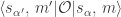. The Wigner–Eckart theorem dictates this probability amplitude’s form. 

and are Hamiltonian eigenstates, thanks to the conservation law. The ETH is an ansatz for the form of —of the elements of matrices that represent operators relative to the energy eigenbasis. The ETH butts heads with the Wigner–Eckart theorem, which also predicts the matrix element’s form.

The Wigner–Eckart theorem wins, being a theorem—a proved claim. The ETH is, as the H in the acronym relates, only a hypothesis.

If conserved quantities are incompatible, we have to kiss the ETH and its thermalization predictions goodbye. But must we set ourselves adrift entirely? Can we cling to no buoy from physics’s best toolkit for quantum many-body thermalization?

No, and yes, respectively. Our clan proposed a non-Abelian ETH for Hamiltonians that conserve incompatible quantities—or, equivalently, that have non-Abelian symmetries. The non-Abelian ETH depends on and on Clebsch–Gordan coefficients—conversion factors between total-spin eigenstates and product states .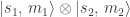

Using the non-Abelian ETH, we proved that many systems thermalize internally, despite conserving incompatible quantities. Yet the incompatibility complicates the proof enormously, extending it from half a page to several pages. Also, under certain conditions, incompatible quantities may alter thermalization. According to the conventional ETH, time-averaged expectation values come to equal thermal expectation values to within corrections, as I explained last month. The correction can grow polynomially larger in the system size, to , if conserved quantities are incompatible. Our conclusion holds under an assumption that we argue is physically reasonable.

So incompatible conserved quantities do alter the ETH, yet another thermodynamic expectation. Physicist Jae Dong Noh began checking the non-Abelian ETH numerically, and more testing is underway. And I’m looking forward to returning to the KITP this fall. Tales do say that paradise is a garden.

View through my office window at the KITP

1Not that married people always trust each other’s judgment.

2The reason is Schur’s lemma, a group-theoretic result. Appendix A of this paper explains the details.