Implied Output Response to Demand Side Shifts in the Friedman Scenario under Local to Potential Assumptions

What does a conventional (estimated) macroeconometric model imply for a sustained 7.7% increase in government consumption and investment as a share of GDP in terms of output.

Table 19 in Friedman (2016) provides a tabulation of annual expenditures implied by his understanding of the Sanders economic plan. Not all of the spending is government consumption and investment — some is government transfers. However, if I assume that the marginal propensity to consume out of these transfers is unit, then the calculation is simplified (in any case, the big expenditures are health care).

Figure 1 depicts the deviation from CBO (January 2016) baseline, as a share of baseline GDP.

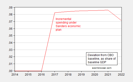
Figure 1: Deviation from CBO baseline in government consumption and investment, as a share of CBO baseline GDP, in Ch.09$, by fiscal year. Source: CBO, Budget and Economic Outlook, 2016-2022 (January 2016); Friedman (2016), Table 19, and author’s calculations.

On average, government spending (will be higher by 7.7 percentage points of baseline GDP). I can just assume constant spending over the sample period, and use the multipliers from a given study to determine the resulting output. In this case, I use the OECD’s New Global Model, described in this 2010 working paper. Here’s a short description of the macroeconometric model:

…Compared with its predecessors, the new model is more compact and regionally aggregated, but gives more weight to the focus of policy interests in global trade and financial linkages. The country model structures typically combine short-term Keynesian-type dynamics with a consistent long-run neo-classical supply-side. While retaining a conventional treatment of international trade and payments linkages, the model has a greater degree of stock-flow consistency, with explicit modelling of domestic and international assets, liabilities and associated income streams. Account is also taken of the influence of financial and housing market developments on asset valuation and domestic expenditures via house and equity prices, interest rates and exchange rates. As a result, the model gives more prominence to wealth and wealth effects in determining longer-term outcomes and the role of asset prices in the transmission of international shocks both to goods and financial markets.

I don’t take into account any of the supply-side effects Friedman outlined (impact on participation rate, for instance). Also, deficits are endogenous, assumed to be stabilized by way of general tax increases, instead of increases in tax progressivity, and taxes on financial transactions. [Specifically in the model, “…the fiscal rule was set to raise direct taxes by approximately one fifth (per annum) of the deviation in the deficit as a percentage of GDP from its baseline path. In the present case, for the countries undertaking fiscal stimulus, this implies more-or-less linear increases in household taxes, rising to be approximately 1 percentage point higher by the fifth year of the shock.”] Hence, the calculation incorporates only the demand side spending effects. Figure 2 shows the deviation from CBO baseline.

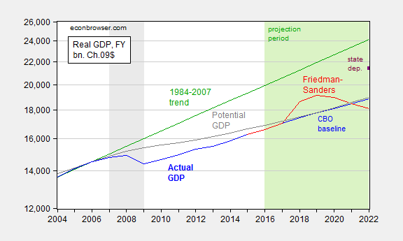
Figure 2: Output, in bn Ch.09$ (blue), output under Friedman scenario using OECD (2010) multipliers (red), output under Friedman scenario using Auerbach and Gorodnichenko (2012) recession multiplier of 1.75 (purple square at 2022), CBO potential GDP (gray) and 1984-2007 trend, all by fiscal year. NBER defined recession dates shaded gray; projection period shaded light green. Source: CBO, Budget and Economic Outlook, 2016-2022 (January 2016); Friedman (2016), Table 19, OECD (2010), Table 3, Auerbach and Gorodnichenko (2012), and author’s calculations.

In this calculation, output reverts fairly quickly toward baseline even with a massive increase in spending. This reflects the neoclassical assumptions built into the model in the long run; implicitly it also reflects the assumption that one is not too far away from potential GDP when the stimulus is undertaken. Hence, as I indicated in this post, in the absence of assuming a flat aggregate supply curve, the assumption regarding the initial extent of economic slack are critical. If indeed the current output gap is -18% or so, then likely the multiplier might be bigger than 1, and perhaps is close to 1.75, as noted in this post. If on the other hand, output is already close to potential in FY2017 (when the spending is assumed to begin), then the multiplier might be closer to 0.5.

So, where you think you will end up depends a lot on where you think you are now…