MTTR: When sample means and power laws combine, trouble follows

Think back on all of the availability-impacting incidents that have occurred in your organization over some decent-sized period, maybe a year or more. Is the majority of the overall availability impact due to:

A large number of shorter-duration incidents, orA small number of longer-duration incidents?

If you answered (2), then this suggests that the time-to-resolve (TTR) incident metric in your organization exhibits a power law distribution. This fact has implications for how good the sample mean of a collection of observed incidents approximates the population (true) mean of the underlying TTR process. This sample mean is commonly referred to as the infamous MTTR (mean-time-to-resolve) metric.

Now, I personally believe that incidents durations are power-law distributed, and, consequently I believe that observed MTTR trends convey no useful information at all.

— Lorin Hochstein (@norootcause.surfingcomplexity.com) 2024-11-30T17:10:05.821Z

But rather than simply asserting that power-law distributions render MTTR useless, I wanted to play with some power-law-distributed data to validate what I had read about power laws. And, to be honest, I wanted an excuse to play with Jupyter notebooks.

Caveat: I’m not a statistician, meaning I’m not a domain expert here. However, hopefully this analysis is simple enough that I haven’t gotten myself into too much trouble here.

You can find my Jupyter notebook here: https://github.com/lorin/mttr/blob/main/power-law.ipynb. You can view it with the images rendered here: https://nbviewer.org/github/lorin/mttr/blob/main/power-law.ipynb

Thinking through a toy example

This post is going to focus entirely on a toy example: I’m going to use entirely made-up data. Let’s consider two candidate distributions for TTR data: a normal tailed distribution and fat-tailed distribution.

The two distributions I used were the Poisson distribution and the Zeta distribution, with both distributions having the same population mean. I arbitrarily picked 15 minutes as the population mean for each distribution.

Poisson

For the normal-tailed distribution, the natural pick would be the Gaussian (aka normal) distribution. But the Gaussian is defined on , and I want a distribution where the probability of a negative TTR is zero. I could just truncate the Gaussian, but instead I decided to go with the Poisson distribution instead, because it doesn’t go negative. Note that the Poisson distribution is discrete where the Gaussian is continuous. The Poisson also has the nice property that it is characterized by only a single parameter (which is called μ in scipy.stats.poisson). This makes this exercise simpler, because there’s one fewer parameter I need to deal with. For Poisson, the mean is equal to μ, so we have μ=15 as our parameter)

Zeta (Zipf)

For the fat-tailed distribution, the natural pick would be the Pareto distribution. The Pareto distribution is zero for all negative values, so we don’t have the conceptual problem that we had with the Gaussian. But it felt a little strange to use a discrete distribution for the normal-tailed case and a continuous distribution for the fat-tailed case. So I decided to go with a discrete power-law distribution, the zeta distribution. This also goes by the name Zipf distribution (of Zipf’s law fame), which is what SciPy calls it: scipy.stats.zipf. This distribution has a single parameter, which SciPy calls a.

I wanted to find the parameter a such that the mean of the distribution was 15. The challenge is that the mean for the zeta distribution is (assume Z is a zeta-distributed random variable):

where ζ(a) is the Riemann zeta function, which is defined as:

Because of this, I couldn’t just analytically solve for a. What I ended up doing was manually executing the equivalent of a binary search to find a value for the parameter a such that the mean for the distribution was close to 15, which was good enough for my purposes.

You can use the stats method to get the mean of a distribution:

>>> from scipy.stats import zipf>>> a = 2.04251395975>>> zipf.stats(a, moments='m')np.float64(15.000000015276777)

Close enough!

Visualizing the distributions

Since these two distributions are discrete, their distributions are characterized by what is called probability mass functions (pmf). The nice thing about pmfs, is that you can interpret the y-axis values directly as probabilities, whereas with the continuous case, you are working with probability density functions (pdfs), where you need to integrate under the pdf over an interval to get a probability.

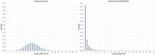
Here’s what the two pmfs look like. I plotted them with the same scales to make it easier to compare them visually.

Click to embiggen

Note how the Poisson pmf has its peak around the mean (15 minutes), where the zeta pmf has a peak at 1 minute and then decreases monotonically.

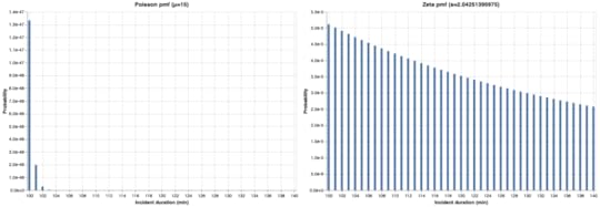
I truncated the x-axis to 40 minutes, but both distributions theoretically extend out to +∞. Let’s take a look at what the distributions looks like further out into the tail, in a window centered around 120 minutes:

Click to embiggen

I didn’t plot the two graphs on the same scale in this case, due to the enormous difference in magnitudes. For the Poisson distribution, an incident of 100 minutes has a probability on the order of , which is fantastically small. For the zeta distribution, an incident of 100 minutes is on the order of , which is 42 orders of magnitude more likely than the Poisson!

You can also see how the zeta distribution falls off much more slowly than the Poisson.

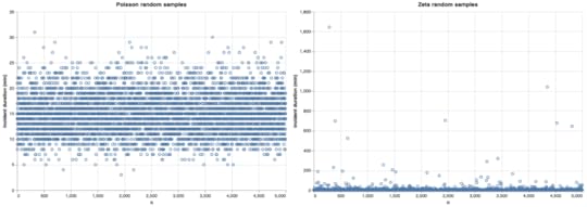
Looking at random samples

I generated 5,000 random samples from each distribution to get a feel for what the distributions look like.

Click to embiggen

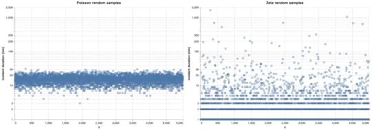
Once again, I’ve used different scales because the ranges are so different. I also plotted them both on a log-scale, this time using the same scale for both.

Click to embiggen

Samples from the Poisson distribution are densest near the population mean (15 minutes). There are a few outliers, but that don’t deviate too far away from the mean.

Samples from the zeta distribution are densest around 1 minute, but spill much further out.

MTTR trends over time

Now, let’s consider that we look at the MTTR (sample mean for our TTR data) at regular intervals, where you can imagine a regular interval to be monthly or quarterly or yearly, or whatever cadence your org uses.

To be concrete, I assumed that we have 25 data points per interval. So, for simplicity, we’re assuming that we have exactly 25 incidents per interval, and we’re computing the MTTR at each interval, which is the average of the TTRs of those 25 samples. With this in mind, let’s look at what the MTTR looks like over time.

I’ll use the same axis for both graphs. I’ve drawn the population mean (15 minutes) as a dashed red line.

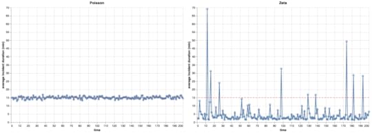Click to embiggen

Which one of these looks more like your incident data?

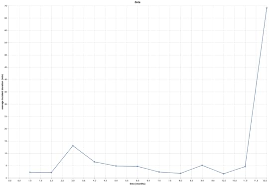
What does the trend convey?

Let’s take a closer look at the data from the zeta samples. Remember that each point represents an MTTR from 25 data points collected over some interval of interest. Let’s pretend these data points represent months, so let’s look at the first 12 of them:

Click to embiggen

I imagine that someone looking at this MTTR would come to the conclusion that:

We did very well in months 1 and 2 (MTTR below 5 minutes!)We saw a regression in month 3 (MTTR about 12 minutes)We saw steady improvements from months 3 to 8 (went back to under 5 minutes)Things didn’t really change from months 8 to 11 (MTTR stayed at or under 5 minutes)We got much, much worse in month 12

The problem with this conclusion is that it’s completely wrong: every single data point was drawn from the same distribution, which means that this graph is misleading: the graph implies changes over time to your TTR distribution which are not there.

Are incidents power-law distributed? What does your data tell you?

This post was just a toy exercise using synthetic data, but I hope it demonstrates how, if incident durations are power-law distributed, looking at MTTR trends over time will lead to incorrect conclusions.

Now, I believe that incident durations are power-law distributed, but I haven’t provided any evidence for that in this post. If you have access to internal incident data in your organization, I encourage that you take a look at the distribution to see whether there’s evidence that it is power-law distributed: is most of the total availability impact from larger incidents, or from smaller ones?

Further reading

Here are a few other sources on this topic that I’ve found insightful.

Incident Metrics in SRE by Štěpán Davidovič

Štěpán Davidovič of Google did an analysis where he looked at real incident data to examine how incident data was distributed, as well as doing Monte Carlo simulations to see whether it was possible to identify whether a change in the true mean (e.g., an intervention that improved TTR) could be identified from the data, and also to see how likely it was to conclude that the system had changed when it actually hadn’t.

He observed that the data doesn’t appear normally distributed. Similar to the analysis I did here, he showed that MTTR trends could mislead people into believing that change had occurred when it hadn’t:

We’ve learned that even without any intentional change to the incident durations, many simulated universes would make you believe that the MTTR got much shorter—or much longer—without any structural change. If you can’t tell when things aren’t changing,
you’ll have a hard time telling when they do.

He published his work this as a freely available O’Reilly mini-book, available here: https://sre.google/resources/practices-and-processes/incident-metrics-in-sre/

Doing statistics under fat tails by Nassim Nicholas Taleb

The author Nassim Nicholas Taleb is… let’s say… unpopular in the resilience engineering community. As an example, see Casey Rosenthal’s post Antifragility is a Fragile Concept. I think Taleb’s caustic style does him no favors. However, I have found him to be the best source on the shortcomings of using common statistical techniques when sampling from fat tailed distributions.

For example, in his paper How Much Data Do You Need? A Pre-asymptotic Metric for Fat-tailedness, he obtains a result that shows that, if you want to estimate the population mean from the sample mean when sampling from a power-law distribution (in this case, an 80/20 Pareto distribution), you need more than times more observations than you would compared to if you were sampling from a Gaussian distribution.

Now, if you have more than one billion times more incidents than the average organization, then MTTR may provide you with a reasonable estimate of the true mean of your underlying TTR distribution! But, I suspect that most readers don’t fall into the over-a-billion-incidents bucket. (If you, do please reach out, I’d love to hear about this!)

Taleb maintains a collection of his papers on this topic here: https://www.fooledbyrandomness.com/FatTails.html

Moving past shallow incident data by John Allspaw

If not MTTR, then what? The canonical answer to this question is this blog post by John Allspaw from back in 2018, entitled Moving Past Shallow Incident Data.

Moving Past Shallow Incident Data

And, of course, I invite readers to continue reading this humble blog on the topic of gathering deeper insights from incidents.