Self-driving Vehicle with Computer Vision

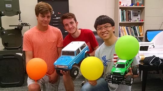High-Altitude Balloon Flight Data Collection System

Self-driving Vehicle with Computer Vision

Physics majors Max Maurer, Spencer Ader, and Ty Carlson (left to right).

In the summer of 2016, I worked with physics major Max Maurer, Spencer Ader, and Ty Carlson on a project that involved object detection, object tracking, and obstacle avoidance for a self-driving vehicle. The vehicle used was a 1/10th scale model of a 1972 Ford Bronco. We added a small USB camera and single-board computer (SBC) to the vehicle to serve as a vision system/brain. Both Raspberry Pi and ODROID XU4 SBCs were tested. The project was a mix of electronics, controls engineering, and image processing. All of the coding was done using Python, with extensive use of the Open Computer Vision (OpenCV) library.

The Vehicle and Electronics

Normally, a radio-controlled car is directly controlled by an onboard radio receiver, which is connected to a steering servo and an electronic speed controller (ESC). When the driver operates the controls on the handheld radio transmitter, the transmitter sends radio signals that are picked up by the receiver. The receiver interprets these signals and sends pulse-width modulated (PWM) signals via wires to control the steering servo and ESC. Since we wanted the vehicle drive itself, we bypassed the radio receiver, connecting the steering servo and ESC directly to an Adafruit PWM/Servo driver. The PWM/Servo driver was, in turn, wired to the onboard computer. This way, instructions could be sent from the computer to the driver, which would then send PWM signals to the steering servo and ESC.

The model Ford Bronco. Note the camera looking through the hole in the windshield.

Inside the Bronco. A Raspberry Pi and USB camera constitute the brain/vision system. In this first iteration, the PWM pins on the Raspberry Pi were connected directly to the steering servo and ESC. However, glitches with the PWM output necessitated using a PWM driver board which was added later.

The USB camera was connected directly to the onboard computer and was mounted to the inside roof of the Bronco, with the lens pointing through a hole cut in the windshield. Captured images were then processed using tools from the OpenCV library. The output of the image processing was used as input for making control decisions. A few different scenarios were investigated: having the vehicle (1) detect and track a known target (brightly colored balls or balloons), (2) follow a winding brick pathway, (3) detect and avoid known obstacles, and (4) avoid unknown obstacles.

A Brief Bit About Color Models

The information that is stored for a color digital image is simply a set of numbers that represent the intensity of red, green, and blue (RGB) light for each pixel. While RGB is the standard format, there is an alternative color model that stores numbers for Hue, Saturation, and Value (HSV). Hue is related to the wavelength of light in the visible spectrum. Saturation refers to the strength of the presence of a color as compared with pure white. Value refers to the lightness or darkness of a color. The HSV color model is often visualized using a cylinder (see below).

The HSV cylinder. (https://commons.wikimedia.org/wiki/User:Datumizer)

The HSV color model is more intuitively representative of the way humans perceive color. For example, imagine we take a picture of a yellow ball that is in full Sun, and then take another picture of the same ball in the shade under a tree. From the first to the second picture, the RGB numbers for each pixel would change in a way that is not necessarily intuitive. However, in the HSV model, the Hue would essentially remain the same, the Saturation may change slightly, and the Value would certainly become darker. This also tends to make HSV suitable for computer vision tasks that detect colored objects, especially in varying lighting conditions.

Detecting a Known Object Based on Color

Our first goal was to have the computer detect a yellow kickball. This was done using the back-projected histogram method. First, an image of the ball is used to construct a 2D histogram with binned values of Hue and Saturation for all of the pixels in the ball. For computational efficiency, the “Value” part of HSV was ignored. This Hue-Saturation (H-S) histogram was then used as a kind of filter for detecting the ball in other images.

An example of an image of the yellow ball and its H-S histogram is shown below. Because every pixel in the image of the ball has similar hues (around 50) and relatively similar saturation (from 150 – 250), the histogram is a sharp peak centered near a hue of 50 and saturation of 200.

Below is another example of an image and its corresponding H-S histogram. Note that this image has a wide variety of hue (greens, blues, etc) and saturation. Therefore, the H-S histogram shows structure at many different combinations of hue and saturation.

In order to determine whether the yellow ball is present in any given image, the image is analyzed pixel by pixel. For each pixel, the hue-saturation pair is compared with the yellow ball’s H-S histogram. The closeness of a given pixel’s hue-saturation pair to the peak in the yellow ball’s H-S histogram is used to generate a number that represents the probability that the pixel from the image is actually from the yellow ball. For example, if the H-S pair for a pixel in the image is (H, S) = (120, 40), this is far away from the yellow ball’s peak at (50, 200), so this pixel is assigned a very low probability of being the ball. However, if the H-S pair in the image is (48, 190), then it is much closer to the peak and is assigned a much higher probability of being the ball.

A probability value is generated for each pixel in the image. These probabilities are then used to construct a corresponding grayscale image known as a histogram back-projection. The back-projection has the same number of pixels (rows and columns) as the original image. Each pixel is assigned a grayscale value, with white being probability of 0 and black being a probability of 1. As an example, below is an image that contains the yellow ball. The grayscale image is the corresponding back-projection produced by the process described above. An algorithm can then be used to find the location of the ball by detecting the cluster of black pixels. Note that the white circle is not a ring of zero probability pixels, but rather a marker placed at the centroid of the black blob.

Tracking an Object of Interest

Once an object of interest can be isolated using a back-projection, OpenCV’s Continuously Adaptive MeanShift (CAMShift) algorithm can be used to track the object in real time. Recall that our object of interest shows up as a dark blob in a back-projection. In each successive video frame, the MeanShift algorithm uses a simple procedure to determine the magnitude and direction of the shift of the dark blob from its location in the previous frame. The continuously adaptive (CA) enhancement of the MeanShift algorithm keeps track of any change in size of the object, usually due to its changing distance from the camera. The information about the location and size of the object is then fed as input into a custom control algorithm to allow the vehicle to track a target at a fixed distance. This required the computer to steer the vehicle in order to keep the target in the center of the field of view, as well as to adjust the vehicle’s speed in order to maintain the following distance. Below is a test video of the vehicle tracking the yellow kickball.

Self-driving vehicle uses OpenCV’s CamShift algorithm and a custom
control algorithm to track a moving target.

We also attached a bright green balloon to the top of a second radio-controlled Ford Bronco to serve as a moving target. The video below is a first-person view from the camera onboard the self-driving vehicle.

First person view from the camera onboard the self-driving vehicle. The target is a green
balloon atop a second radio-controlled Ford Bronco. The blue square shows the location
and size of the object detected by OpenCV’s CamShift algorithm.

Follow the “Red” Brick Road!

With the ability to isolate and track an object of interest based on color, it was now a relatively simple matter to have the vehicle follow a winding pathway. The path we used was made of different shades of red brick. We stitched together a composite image of the various types of brick and used it to generate an H-S histogram. A histogram back-projection could then generated, showing the location of the brick path (see below). Note here that the grayscale colors are reversed; white pixels are a probability of 1 and black pixels are a probability of 0.

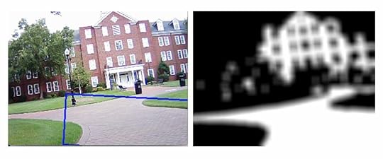
The geometric center of the brick material was then calculated, and the computer issued steering commands to keep this point in the center of the field of view. As you can tell from the above image, not only was the process successful at showing the brick path, but it showed the brick buildings as well. To remedy this problem, we had to mask off the top portion of the back-projection when computing the geometric center of the brick path. Below is a test video taken of the self-driving vehicle as it attempts to stay on the brick path.

Due to the vehicle’s short stature, the camera was very close to the ground making the brick fill up most of the bottom portion of the field of view. As a result of this loss of perspective cues, the vehicle was sometimes not able to tell if it was driving along the center of the path or at an angle toward the edge of the path. At times, the vehicle ended up driving at a right angle toward the edge of the path. In these cases, the edge of the path was a horizontal line across the field of view of the camera (see below).

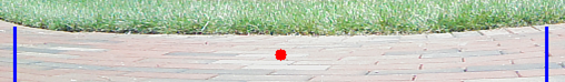Edge case: Heading straight for the edge of the path. Because the center of the brick path is in the center of the field of view, the vehicle continues to drive straight ahead, eventually running into the grass.

Unfortunately, this meant that the center of the brick path was in the middle of the image, so the vehicle just kept driving straight toward the edge of the path, eventually ending up in the grass. To solve this problem, we had the algorithm keep track of the percentage of the image that was brick. As the vehicle drove toward the edge of the path, more of this area would become filled with grass and the percentage of brick would shrink. At a certain threshold, the vehicle was programmed to begin slowing down and make a sharp turn in one direction to stay on the path.

Avoiding Known Obstacles

To incorporate obstacle avoidance into the self-driving vehicle’s capabilities, we took inspiration from the behavior of electrically charged particles. The characteristics of this behavior are well suited for developing a model of obstacle avoidance:

Like electrical charges (e.g. + and +) repel and unlike charges (+ and -) attract.The closer charges are to one another, the more strongly they attract or repel.The greater the magnitude of the charges, the more strongly they attract or repel.The overall (or net) force experienced by a single charge is a linear superposition of the forces caused by each of the charges surrounding it.

Using Item #1 in the list above, we think of the vehicle as having a positive electric charge. Targets are then considered to have a negative charge, while obstacles are considered to have a positive charge. As a specific example, consider the image below, which is taken from the self-driving vehicle’s camera and shows a single target (green balloon) and a group of obstacles (red, blue, and orange balloons).

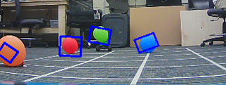First person view from the self-driving vehicle’s camera showing a target (green balloon) and three obstacles (orange, red, and blue balloons). The vehicle is a positive charge and the target is a negative charge. Therefore, the vehicle is attracted to the target. The obstacle balloons have a positive charge. Therefore, these balloons and the vehicle are repelled from one another.

For the target, the algorithm calculates a steering command that would tend to bring the target toward the center of the field of view (attract). Because the green balloon is close to the center of the image above, this would only require a small left turn. For an obstacle, the computer calculates a steering command that would cause the obstacle to move away from the center of the field of view (repel). Since the blue balloon is close to the center of the image, this would require a sharp turn to the left. The red balloon would require a slightly less sharp turn to the right. The orange balloon would require a fairly weak turn to the right. The specific steering commands are determined using graphs called steering curves. You can read about the steering curves in detail here if you are interested.

It is probably obvious that the vehicle can only receive one steering command to position the wheels. So, what happens when there are multiple objects like in the situation described above? This is where the principle of linear superposition (Item #4 on the list above) comes into play. For the sake of argument, let’s assign some arbitrary numerical values for the steering commands to see how this works. Let’s say a neutral steering command (no turn) is 0, a left turn command is a negative number, and a right turn command is a positive number. The sharper the turn required, the greater the magnitude of the command. So, for example, a very weak left turn might be -10, while a very strong right turn might be +100. In the image above, the green target would require a weak left turn to bring it to the center of the field of view. Using the letter ‘S’ to denote a steering command, let’s say this steering command is Sgreen = -10. Because it is close to the center, the blue obstacle requires a strong left turn to avoid. Let’s say Sblue = -80. The red balloon is a little farther away from the center, so perhaps the steering command to avoid it would be a moderate right turn of Sred = +60. Finally, the orange obstacle is close to the left edge, so it only requires a weak right turn of Sorange = +10 to avoid. In order to determine the net steering command to be sent to the servo, we take the superposition of these separate steering commands:

Snet = Sgreen + Sblue + Sred + Sorange = (-10) + (-80) + (+60) + (+10) = -20

So, the net steering command is -20. This is the command we actually send to the steering servo. This relatively weak left turn makes sense, as it sets a course between the red and blue obstacles, heading for the green target. Because the orange obstacle is so far to the left, this command will likely not bring us too close to it. In this way, the superposition helps the vehicle navigate its way through a field of obstacles.

Thus far, we have taken into account how close the object is to the center of the field of view when determining a steering command, however we have not yet considered the actual distance between the vehicle and object (Item #2 in the list above). Because we know the actual size of an object (i.e. balloon), we can use this along with its apparent size in the image to estimate the distance to it and use this information to place greater weight on the steering commands for nearby objects and less weight on the steering commands for far away objects. If we represent the weighting factor, w, as a function of distance, d, for object i as wi(di), then the distance weighted net steering command for n objects is:

Snet = w1(d1)*S1 + w2(d2)*S2 + . . . + wn(dn)*Sn

The net steering command is thus a weighted average of the individual steering commands for all of the objects in the vehicle’s field of view. Below are a some test videos that show the vehicle using this model to avoid obstacles and reach a target. The target is a green balloon attached to a small green RC vehicle.

Although we did not incorporate Item #3 from the list above, one could do so by imagining that different obstacles have different inherent levels of danger. For example, perhaps a red balloon is more dangerous than a blue balloon. Therefore, one could modify the weighting factors such that steering commands to avoid red balloons carry a greater weight than steering commands to avoid blue balloons.

Avoiding Unknown Obstacles Using Optical Flow

The final challenge was to have the vehicle avoid obstacles that were not known in advance. That is, we wanted the vehicle to be able to avoid any object placed in its path, not just brightly colored balloons. To accomplish this, optical flow was used to ???. Optical flow refers to the apparent movement of objects in a field of view due to the relative motion between the objects and the observer. This apparent motion could be due to the motion of the objects in the scene, the motion of the observer, or both. Consider the image below, which shows the view of a passenger looking out the window of a train. In the left frame the train is at rest, while in the right frame the train is moving to the right.

Because of parallax, objects closer to the train appear to move by faster (hence the blur), while distant objects appear to move by more slowly. If we place arrows on the objects in the scene to depict their apparent motion, with the arrowhead showing the direction and the length representing the speed, this would look something like the image below.

The red arrows visually depict the direction and speed of the apparent motion of objects in the passenger’s field of view. The collection of arrows is called an optical flow field.

One of OpenCV’s dense optical flow methods, which is based on Farneback’s algorithm , was used to produce optical flow fields for the scene viewed by the self-driving vehicle. An example is shown below. There are no arrowheads in this image, so note that the arrows begin at the blue dots and point along the red lines.

One shortcoming of using this method directly on images without any preprocessing (segmentation, etc) is that it is not possible for the routine to detect the motion of pixels in areas with little to no texture. In the image above, this is revealed in smooth areas like the large white patches of walls, ceiling, and floor. However, where there are distinct edges and texture — like around posters, doors, or even reflections of lights in the floor — the routine can detect the motion of pixels, hence the presence of optical flow vectors in these locations. In our tests, we used obstacles that had some level of surface texture to alleviate this issue.

How is the optical flow field useful in an obstacle avoidance framework? Objects that are farther away from the vehicle will have lower apparent speeds and therefore shorter optical flow vectors, while objects that are closer to the vehicle will have higher apparent speeds and therefore longer optical flow vectors. Rather than attempt to isolate individual objects, we simply divided the image in half with a vertical line. We then summed the lengths of the optical flow vectors on each side. Whichever side had the highest total was assumed to contain closer obstacles. Therefore, the vehicle was instructed to steer away from the side with the higher total.

The image below is from the point of view of the self-driving vehicle. The yellow numbers show the overall sums of the optical flow vector lengths for the left side (669) and right side (967) of the image. The large book in the foreground is contributing significantly to the higher total on the right. At this instant, the vehicle would be sent a steering command to turn to the left by an amount proportional to the difference between the total sums.