Statistopia

When is an Average Not an Average?

Now and then, one reads that the average American is a woman.  There are certain construals under which this might be true; but social criticism is not today my theme.  My theme is, yes, wait for it: statistics, more fun than which is impossible to have sitting down.  

Now, in fact, what folks usually mean is that a slight majority of Americans are women.  This is largely because teenaged boys are allowed to drive.  OK, that was insensitive.  But the fact is that mortality is greater among men than among women.  This is why auto insurance premiums were once higher for boys than for girls, before Our Government, in its on-going search for Fairness decreed that insurance companies must no longer take into account the real world.  Rates then rose for young women drivers, providing an opening for a discussion about the true meaning of social justice and fairness.  Or would, if that were what this is all about.  

But to say that the "average American" is a woman is to distort the meaning of average.  In one sense, the category Woman being the more numerous, it is a sort of mode, but the axis of categories is, well, categorical, not numerical.  The mode is the most frequent value in a sample or population.  If the most frequent value is 3.14159, we would have pi a la mode.  But the arithmetic average is what we mean.  (Pun intended!)  The arithmetic average American has one testicle and one ovary.  Take a sample of people, count the number of testicles on each - look, how you go about doing so is your own business - and divide the sum by the sample size.  It will actually average just under one, because, well, let's not get into that.  

An old statistician's joke runs "If you stick your head in the oven and feet in the freezer, on the average, you're comfortable."  Which is why most statisticians have not quit their day jobs and headed off for Vegas and the comedy clubs.  But the point is pointed.  An average is a measure of central tendency, and not all algorithmically calculated averages measure a central tendency.  Sometime, there just isn't one, and in that sense, there is no average.  What is the central tendency of males and females.  What would be the number of Persons in the Hypostatic Union of the Godhead if the sample included traditional Christians (3), muslims and Jews (1), Taoists and neopagans (2), and atheists (0).  One can easily imagine an evening newsreader and the blogosphere soberly reporting that in popular opinion God now contains 2.1 persons, and speculating on the meaning of this for the future of theology.  Aside from indicating that newsreaders have no future as theologians, it is meaningless drivel.  But I digress.  

In static populations, distinct strata may each have its distinct mean value.  An overall mean would be meaningless, as above.  In fact, the purpose of many statistical tests, like One-Way ANOVA (which would be a great name for a test pilot), is to discover if several strata have a common mean or not.  

In dynamic processes, the distinct strata may be subsumed within the periodic samples or may appear as distinct fluctuations or shifts from time to time.  In this case, calculating a constant mean for the series can be a fatuous exercise, though often done simply to provide a benchmark against which to view the fluctuations and to test the null hypothesis that the mean value is constant for the series.  
 

Note that while the grand mean is 7.32 (in coded values: this is real data), there is no sense in which we might say "The pasting process maintained a process level of 7.32."  Maybe it was briefly true at 4:30.  There are clear changes in the process level.  Of the first twelve means, all but two were below the grand mean.  Of the second twelve means, all but one were above the grand mean.  We conclude that some action was taken around 4:00 PM that raised the overall average.  This turned out to be a change in the density of the lead oxide paste that was being metered into the machine.  There had been a change in the paste mill and the same volume of paste was resulting in heavier paste weights on the grids.  

A closer inspection reveals something more interesting: a "leap" in the mean value at each hourly sample.  Between the hours, there is much less variation.  This was due to the machine operator diligently adjusting the machine just before the QC patrol inspector was scheduled to come by for the control sample.  (We were doing a special study, and thus in some odd sense "invisible.")  

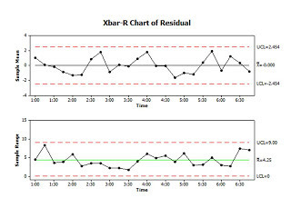
 Now suppose we wanted to know about the machine's capability regardless of these two assignable causes - the change in paste density and the operator's well-intended tampering?  The way we would do this would be to calculate the mean of each hour and plot not the sample means but the deviation of the sample means from its own hourly mean.  Such deviations are technically called "deviations" (and, with a bit of math, compared to a "standard" deviation); but they are also commonly called "residuals." The chart of residuals looks like this:

As you can see, it is "in control," meaning the long term variation is no greater than the short term variation (everything fits between the 3-sigma limits) and the grand mean really does look like a central tendency.  IOW, once we have addressed the oxide density and the operator adjustments the process becomes a nicely predictable stationary time series.  It also plots as a straight line on normal probability paper, and so is consistent with the assumption that the residuals vary normally around a mean of zero.  This is a condition at which statisticians get all dreamy-eyed and get their mojo working.  With normal residuals averaging 0, one may pursue that ANOVA hereabove mentioned and perform all sorts of 19th century tests of significance. 

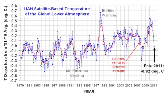
With this in mind, interested readers are welcomed to examine the following time series:

These are satellite-based temperatures of the lower atmosphere.  Dr. Roy Spencer describes the actual measurements with admirable concision.  

NOAA satellites have been carrying instruments which measure the natural microwave thermal emissions from oxygen in the atmosphere. The signals that these microwave radiometers measure at different microwave frequencies are directly proportional to the temperature of different, deep layers of the atmosphere. Every month, John Christy and I update global temperature datasets that represent the piecing together of the temperature data from a total of eleven instruments flying on eleven different satellites over the years. As of early 2011, our most stable instrument for this monitoring is the Advanced Microwave Sounding Unit (AMSU-A) flying on NASA’s Aqua satellite and providing data since late 2002. ... [T]he satellite measurements are not calibrated in any way with the global surface-based thermometer record of temperature. They instead use their own on-board precision redundant platinum resistance thermometers calibrated to a laboratory reference standard before launch.

For reasons unknown, "climate scientists" call their residuals "anomalies."  The data points are monthly, and each month is compared to the mean value for that month for 1981-2010.  That is, a mean is computed for Jan 81, Jan 82, ..., Jan 10, and each Jan average is compared to this grand mean.  And so on for each month.  The result is to filter out the summer-winter temperature changes and center the chart on 0.  This is what we did above when we did hourly averages to eliminate the end-of-hour adjustment by the operator.  Thus, there is no seasonal fluctuation in the residual time series.

There are no control limits because climate scientists have evidently never heard of Walter Shewhart and his seminal work on dynamic statistics.  Instead, we see constant means, linear regressions, linear extrapolations, and the like.  Yet the data clearly indicates there is more than one regime in the data.  There are spike events - highly touted when they spike up, ignored when they spike down.  (Skeptics tout the down-spikes.)  There is a cycle of approximately 3.75 years (irregular: most often 3-5 years between peaks; and two peaks were suppressed by something).  The last spike event at the end of the chart resembled that of the 1998 El Nino.  What the record is not is:

a) constant; or

b) a steady linear trend upward correlating with CO2.  

My impression: there are assignable causes in the process not yet identified.  By not including them in the model, the fluctuations due to them are assigned to the included factors, thus exaggerating their influence.  This is the hazard of starting with a model and working toward the data, rather than starting from the data and identifying assignable causes.  When the climate then does the unexpected, the unpredicted, one must run about modifying the model to accommodate it.