Paul Gilster's Blog, page 3

New Model to Prioritize the Search for Exoplanet Life

Our recent focus on habitability addresses a significant problem. In order for astrobiologists to home in on the best targets for current and future telescopes, we need to be able to prioritize them in terms of the likelihood for life. I’ve often commented on how lazily the word ‘habitable’ is used in the popular press, but it’s likewise striking that its usage varies widely in the scientific literature. Alex Tolley today looks at a new paper offering a quantitative way to assess these matters, but the issues are thorny indeed. We lack, for instance, an accepted definition of life itself, and when discussing what can emerge on distant worlds, we sometimes choose different sets of variables. How closely do our assumptions track our own terrestrial model, and when may this not be applicable? Alex goes through the possibilities and offers some of his own as the hunt for an acceptable methodology continues.

by Alex Tolley

Artist illustrations of explanets in the habitable zone as of 2015. None appear to be illustrated as possible hanbitable worlds. This has changed in the last decade. Credit: PHL @ UPR Arecibo (phl.upr.edu) January 5, 2015 Source [1]

We now know that the galaxy is full of exoplanets, and many systems have rocky planets in their habitable zones (HZ). So how should we prioritize our searches to maximize our resources to confirm extraterrestrial life?

A new paper by Dániel Apai and colleagues of the Quantitative Habitability Science Working Group, a group within the Nexus for Exoplanet System Science (NExSS) initiative, looks at the problems hindering our quest to prioritize searches of the many possible life-bearing worlds discovered to date and continuing to be discovered with new telescope instruments.

The authors state that the problem we face in the search for life is:

“A critical step is the identification and characterization of potential habitats, both to guide the search and to interpret its results. However, a well-accepted, self-consistent, flexible, and quantitative terminology and method of assessment of habitability are lacking.”

The authors expend considerable space and effort itemizing the problems that have accrued: Astrobiologists and institutions have never defined “habitable” and “habitability” rigorously, even confounding “habitable” with “Habitable Zone” (HZ), and using “habitable” and “inhabited” almost interchangeably. They argue that this creates problems for astrobiologists when trying to plan how to develop strategies when determining which exoplanets are worth investigating and how. Therefore, defining terminology is important to avoid confusion. As the authors point out, researchers often assume that planets in the HZ should be habitable and those outside its boundaries uninhabitable, even though both assertions are untrue.

[I am not clear that the first assertion is claimed without caveats, for example, the planet must be rocky and not a gaseous world, such as a mini-Neptune.]

As our knowledge of exoplanets is data poor, it may not be possible to define whether a planet is habitable based on the available information, which leads to the imprecision of the term “habitable”. In addition, not only has “habitable” not been well-defined, but neither have the requirements for life been defined, which is more restrictive than the loose requirement for surface liquid water.

Ultimately, the root of the problem that hampers the community’s efforts to converge on a definition for habitability is that habitability depends on the requirements for life, and we do not have a widely agreed-upon definition for life.

The authors accept that a universal definition of life may not be possible, but that we can, however, determine the habitat requirements of particular forms of life.

The authors’ preferred solution is to model habitability with joint probability assessments of planetary conditions with already acquired data, and extended with new data. This retains some flexibility in the use of the term “habitable” in the light of new data.

Figure 1 below illustrates the various qualitative approaches to defining habitability. Adhering to any single definition is not possible for a universal definition. The paper suggests that a better approach is to use quantitative methods that are both rigorous, yet flexible in the light of new data and information.

Figure 1. Various approaches to defining “habitable”. Any single definition for “habitability” fails to meet the majority of the requirements.

The equation below illustrates the idea of quantifying the probability of a planet’s habitability as a joint probability of the known criteria:

The authors use the joint probability of the planet being habitable. For example, it is in the HZ, is rocky, and has water vapor in the atmosphere. Clearly, under this approach, if water vapour cannot be detected, the probability of habitability declines to zero.

Perhaps of even greater importance, the group also looks at habitability based on whether a planet supports the requirements for known examples of terrestrial life, whose requirements vary considerably. For example, is there sufficient energy to support life? If there is no useful light from the parent star in the habitat, energy must be supplied by geological processes, leading to the likelihood that only anaerobic chemotrophs could live under those conditions, for example, as hypothesized in dark, glacial-covered subsurface oceans..

The authors include more carefully defined terms, including: Earth-like life. Rocky Planet, Earth-Sized Planet, Earth-Like Planet, Habitable Zone, Metabolisms, Viability Model, Suitable Habitat for X, and lastly Habitat Suitability which they defined as:

The measure of the overlap between the necessary environmental conditions for a metabolism and environmental conditions in the habitat.

Because of the probability that life (at least some species of terrestrial life) will inhabit a planet, the authors suggest a framework where the Venn diagram of the probability of a planet being habitable intersects with the probability that the requirements are met for specific species of terrestrial life.

The Quantitative Habitability Framework (QHF) is shown in Figure 2 below.

Figure 2. Illustration of the basis of the Framework for Habitability: The comparison of the environmental conditions predicted by the habitat model and the environmental conditions required by the metabolism model.

The probability of the viability of an organism for each variable is a binary value of 0 for non-viability and 1 for viability. For archaea and temperature, this is:

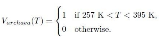
The equation means that the probability of viability of the archaea at temperature T in degrees Kelvin is 1 if the temperature is between 257 K ( -16 °C) and 395 K (122 °C). Otherwise 0 if the temperature is outside the viable range. (Ironically, this is imprecise, as it is for a species of archaean methanogen extremophile, not all archaeans.)

This approach is applied to other variables. If any variable probability is zero, the joint probability of viability becomes 0.

The figure below shows various terrestrial organism types, mostly unicellular, with their known temperature ranges for survival. The model therefore allows for some terrestrial organisms to be extant on an exoplanet, whilst others would not survive.

Figure 3. Examples of temperature ranges for different types of organisms, taken for species at the extreme ranges of survival in the laboratory.

To demonstrate their framework, they work through models for archaean life on Trappist 1e and Trappist 1f, cyanobacteria on the same 2 planets, methanogens (that would include archaea) in the subsurface of Mars, and the subsurface ocean of Enceladus.

Figure 4 below shows the simplified model for archaea on Trappist 1e. The values and standard deviations used for the priors are not all explained in the text. For example, the mean surface pressure is set at 5 Bar for illustrative purposes, as no atmosphere has been detected for Trappist-1e. The network model for the various modules that determine the viability of an archaean is mapped in a). Only 2 variables, surface temperature and pressure, determine viability of the archaean prokaryotes in the modeled surface temperature. In more sophisticated models, this would be a multidimensional plot perhaps using principal component analysis (PCA) to show a 3D plot. The various assumed (prior) and calculated (result) values and their assumed distributions are shown as charts in b). The plot of viability (1) and non-viability (0) for surface temperature and pressure is shown in the 3D plot c. The distributions indicate the probability of suitability of the habitat.

Figure 4. QHF assessment of the viability of archaea/methanogens in a modeled TRAPPIST-1e-like planet’s surface habitat. a: Connections between the model modules. Red are priors, blue are calculated values, green is the viability model. b: Relative probability distributions of key parameters. c: The distribution of calculated viability as a function of surface temperature and pressure. The sharp temperature cutoff at 395K separates the habitat as viable or not.

The examples are then tabulated to show the probabilities of different unicellular life inhabiting the various example worlds.

As you can see, the archaea/methanogens on Trappist 1f have the highest probability of being present inhabiting that world if we assume terrestrial life represents good examples. Therefore, Trappist 1f would be prioritized given the information currently available. If spectral data suggested that there was no water in Trappist 1f’s atmosphere, this would reduce, and possibly eliminate, this world’s habitability probability, and with it the probability of it meeting the requirement of archaean life and hence reducing the overlap in the habitability and life requirement terms to nil.

My Critique of the Methodology

The value of this paper is that it goes beyond the usual “Is the exoplanet habitable?” with the usual caveats about habitability that apply under certain conditions, usually atmospheric pressure and composition. The habitable zone (HZ) around a star is calculated for the range of distances from the star where, with an ideal atmosphere composition and density, on a rocky surface, liquid water could be found. Thus, early Mars, with a denser atmosphere, could be habitable [2], and indeed, the evidence is that water was once present on the surface. Venus might also once have been habitable, positioned at the inner edge of our sun’s HZ, before a runaway greenhouse made the planet uninhabitable.

The concept of NASA’s “Follow the water” mantra is a first step, but this paper then points out this is only part of the equation when deciding the priority of expending resources on observing a prospective exoplanet for life. The Earth once had an anoxic atmosphere, making Lovelock’s early idea that gases in disequilibrium would indicate life, which quickly became interpreted as free oxygen (O2) and methane (CH4), largely irrelevant during this period before oxygenic photosynthesis changed the composition of the atmosphere.

Yet Earth was living within a few hundred million years after its birth, with organisms that predated the archaea and bacteria kingdoms [4]. Archaea are often methanogens, releasing CH4 into the early atmosphere at a rate exceeding that of geological serpentinization. Their habitat in the oceans must have been sufficiently temperate, albeit some are thermophilic, living in water up to 122 centigrade but under pressure to prevent boiling. If the habitability calculations include the important variables, then their methodology offers a rigorous way to determine the probability of particular terrestrial life on a prospective exoplanet.

The problem is whether the important variables are included. As we see with Venus, if the atmosphere was still Earthlike, then it might well be a prospective target. Therefore, an exoplanet on the inner edge of its star’s HZ might need to have its atmosphere modeled for stability, given the age of its star, to determine whether the atmosphere could still be earthlike and therefore support liquid water on the surface.

However, there may be other variables that we have repeatedly discussed on this website. Is the star stable or does it flare frequently? Does the star emit hard UV and X-rays that would destroy life on the surface by destroying organic molecules? Is the star’s spectrum suited for supporting photosynthesis, and if not, does it allow or prevent chemotrophs to survive? For complex life, is a large moon needed to keep the rotational axis relatively stable to prevent climate zones and circulation patterns from changing too drastically? Is the planet tidally locked, and if so, can life exist at the terminator, as we have no terrestrial examples to evaluate? The Ramirez paper [3] includes his modeling of Trappist 1e, using the expected synchronization of its rotation and orbital period, resulting in permanently hot and cold hemispheres.

While the authors suggest that the analysis can extend beyond species to ecosystems, and perhaps a biosphere, we really don’t know what the relevant variables are in most cases. Unicellular organisms are sometimes easily cultured in a laboratory, but most are not. We just don’t know what conditions they need, and whether these conditions exist on the exoplanet. It may be that the equation variables may be quite large, making the analyses too unwieldy to be worth doing to evaluate the probability of some terrestrial life form inhabiting the exoplanet.

A further critique is that organisms rarely can exist as pure cultures except in a laboratory setting with ideal culture media. Organisms in the wild exist in ecosystems, where different organisms contribute to the survival of others. For example, bacterial biofilms often comprise different species in layers allowing for different habitats to be supported, from anaerobes to aerobes.

The analysis gamely looks at life below the surface, such as lithophilic life 5 km below the surface of Mars, or ocean life in the subsurface Enceladan ocean. But even if the probability in either case was 100% that life was present, both environments are inaccessible compared to other determinants of life that we can observe with our telescopes. This would apply to icy moons of giant exoplanets, even if future landers established that life existed in both Europan and Enceladan subsurface oceans.

What about exoplanets that are not in near circular orbits, but more eccentric, like Brian Aldiss’ fictional “Heliconia”? How to evaluate their habitability? Or circumbinary planets where the 2 stars are creating differing instellation patterns as the planet orbits its close binary?. Lastly, can tidally locked exoplanets support life only at the terminator that supports the range of their known requirements, such as Ramirez’ modeling of Trappist 1e?

An average surface temperature does not cover either the extremes, for example the tropics and the poles, nor that water is at its densest at 277K (4 °C), ensuring that there is liquid water even when the surface is fully glaciated above an ocean. Interior heat can also ensure liquid water below an icy surface, and tidal heating can contribute to heating even on moons that have exhausted their radioactive elements. If the Gaia hypothesis is correct, then life can alter a planet to support life even under adverse conditions, stabilizing the biosphere environment. The range of surface temperatures is covered by the Gaussian distribution of temperatures as shown in Figure 4 b.

Lastly, while the joint probability model with Monte Carlo simulation to estimate the probability of an organism or ecosystem inhabiting the exoplanet is a relatively computationally lightweight model, it may not be the right approach with more variables added to the mix. The probabilities may be disjoint with a union of different subsets of variables with joint probabilities. In other words, rather than “and” intersections of planet and organism requirement probabilities, there may be an “or” union of probabilities. The modeled approach may prove brittle and fail, a known problem of such models, which can be alleviated to some extent by using only subsets of the variables. Another problem I foresee is that a planet with richer observational data may score more poorly than a planet with few data-supported variables, simply due to the joint probability model.

All of which makes me wonder if the approach really solves the terminology issue to prioritize exoplanet life searches, especially if a planet is both habitable and potentially inhabited. It is highly terrestrial-centric, as we would expect, as we have no other life to evaluate. If we find another life on Earth, as posited by Paul Davies’ “Shadow Biosphere,” [4] this methodology could be extended. But we cannot even determine the requirements of extinct animals and plants that have no living relatives, but flourished in earlier periods on Earth. Which species survived when Earth was a hothouse in the Carboniferous, or below the ice during the global glaciations? Where were those conditions outside the range of extant species? For example, post-glacial humans could not survive during the Eocene thermal maximum.

For me, this all boils down to whether this method can usefully help determine whether an exoplanet is worth observing for life. If an initial observation ruled out an atmosphere like any of those Earth has experienced in the last 4.5 billion years, should the search for life be immediately redirected to the next best target, or should further data be collected, perhaps to look for gases in disequilibrium? While I wouldn’t bet that Seager’s ‘MorningStar’ mission to look for life on Venus will find anything, if it did turn up microbes in the acidic atmosphere’s temperate zone, that would add a whole new set of possible organism requirements to evaluate, making Venus-like exoplanets viable targets for life searches. If we eventually find life on exoplanets with widely varying conditions, with ranges outside of terrestrial life, would the habitat analyses then have to test all known life from a catalog of planetary conditions?

But suppose this strategy fails, and we cannot detect life, for various reasons, including instrumentation limits? Then we should fall back on the method I last posted on, which reduces the probability of extant life on an exoplanet, but leaves open the possibility that life will eventually be detected.

The paper is Apai et al (2025)., “A Terminology and Quantitative Framework for Assessing the Habitability of Solar System and Extraterrestrial Worlds,” in press at Planetary Science Journal. Abstract.

References

1. Schulze-Makuch, D. (2015) Astronomers Just Doubled the Number of Potentially Habitable Planets. Smithsonian Magazine, 14 January 2015.
https://www.smithsonianmag.com/air-space-magazine/astronomers-just-doubled-number-potentially-habitable-planets-180953898/

2. Seager, S. (2013) “Exoplanet Habitability,” Science 340, 577.
doi: 10.1126/science.1232226

3. Ramirez R., (2024). “A New 2D Energy Balance Model for Simulating the Climates of Rapidly and Slowly Rotating Terrestrial Planets,” The Planetary Science Journal 5:2 (17pp), January 2024
https://doi.org/10.3847/PSJ/ad0729

4. Tolley, A. (2024) “Our Earliest Ancestor Appeared Soon After Earth Formed” https://www.centauri-dreams.org/2024/08/28/our-earliest-ancestor-appeared-soon-after-earth-formed

5. Davies P. C. W. (2011) “Searching for a shadow biosphere on Earth as a test of the ‘cosmic imperative,” Phil. Trans. R. Soc. A.369624–632 http://doi.org/10.1098/rsta.2010.0235

A Sedna Orbiter via Nuclear Propulsion

When you’re thinking deep space, it’s essential to start planning early, at least at our current state of technology. Sedna, for example, is getting attention as a mission target because while it’s on an 11,000 year orbit around the Sun, its perihelion at 76 AU is coming up in 2075. Given travel times in decades, we’d like to launch as soon as possible, which realistically probably means sometime in the 2040s. The small body of scientific literature building up around such a mission now includes a consideration of two alternative propulsion strategies.

Because we’ve recently discussed one of these – an inflatable sail taking advantage of desorption on an Oberth maneuver around the Sun – I’ll focus on the second, a Direct Fusion Drive (DFD) rocket engine now under study at Princeton University Plasma Physics Laboratory. Here the fusion fuel would be deuterium and helium-3, creating a thermonuclear propulsion thruster that produces power through a plasma heating system in the range of 1 to 10 MW.

DFD is a considerable challenge given the time needed to overcome issues like plasma stability, heat dissipation, and operational longevity, according to authors Elena Ancona and Savino Longo (Politecnico di Bari, Italy) and Roman Ya. Kezerashvili (CUNY), the latter having offered up the sail concept mentioned above. See Inflatable Technologies for Deep Space for more on this sail. A mission to so distant a target as Sedna demands evaluation of long-term operations and the production of reliable power for onboard instruments.

Nonetheless, the Princeton work has captured the attention of many in the space community as being one of the more promising studies of a propulsion method that could have profound consequences for operations far from the Sun. And it’s also true that getting off at a later date is not a showstopper. Sedna spends about 50 years within 85 AU of the Sun and almost two centuries within 100 AU, so there is an ample window for developing such a mission. Some mission profiles for closer targets, such as Titan and various Trans-Neptunian objects, and other Solar System destinations are already found in the literature.

Image: Schematic diagram of the Direct Fusion Drive engine subsystems with its simple linear configuration and directed exhaust stream. A propellant is added to the gas box. Fusion occurs in the closed-field-line region. Cool plasma flows around the fusion region, absorbs energy from the fusion products, and is then accelerated by a magnetic nozzle. Credits [5].

The Direct Fusion Drive produces electrical power as well as propulsion from its reactor, and shows potential for all these targets as well as, obviously, more immediate destinations like Mars. What is being called a ‘radio frequency plasma heating’ method uses a magnetic field that contains the hot plasma and ensures stability that has been hard to achieve in other fusion designs. Deuterium and tritium turn out to be the most effective fuels in terms of energy produced, but the deuterium/helium-3 reaction is aneutronic, and therefore does not require the degree of shielding that would otherwise be needed.

The disadvantages are also stark, and merit a look lest we get overly optimistic about the calendar. Helium-3 and deuterium require reactor temperatures as much as six times higher than demanded with the D-T reaction. Moreover, there is the supply problem, for the amount of helium-3 available is limited:

The D-3He reaction is appealing since it has a high energy release and produces only charged particles (making it aneutronic). This allows for easier energy containment within the reactor and avoids the neutron production associated with the D-T reaction. However, the D-3He reaction faces the challenge of a higher Coulomb barrier [electrostatic repulsion between positively charged nuclei], requiring a reactor temperature approximately six times greater than that of a D-T reactor to achieve a comparable reaction rate.

So what is the outline of a Direct Fusion Drive mission if we manage to overcome these issues? The authors posit a 1.6 MW DFD, working the numbers on the Earth escape trajectory, interplanetary cruise (a coasting phase) and final maneuvers at target. In an earlier paper, Kezerashvili has shown that the DFD option could reach the dwarf planet Eris in 10 years. The distance of 78 AU matches with Sedna’s perihelion, meaning Sedna itself could be visited in roughly half the time calculated for any other propulsion system considered.

Bear in mind that it has taken New Horizons 19 years to reach 61 AU. DFD is considerably faster, but notice that the mission outlined here assumes that the drive can be switched on and off for thrust generation, meaning a period of inactivity during the coasting phase. Will DFD have this capability? The authors also evaluate a constant thrust profile, with the disadvantage that it would require additional propellant, reducing payload mass.

In the thrust-coast-thrust profile, the authors’ goal is to deliver a 1500 kg payload to Sedna in less than 10 years. The authors calculate that approximately 4000 kg of propellant would be demanded for the mission. The DFD engine itself weighs 2000 kg. The launch mass bumps up to 7500 kg, all varying depending on instrumentation requirements. From the paper:

The total ∆V for the mission reaches 80 km/s, with half of that needed to slow down during the rendezvous phase, where the coasting velocity is 38 km/s. Each maneuver would take between 250 and 300 days, requiring about 1.5 years of thrust over the 10-year journey. However, the engine would remain active to supply power to the system. The amount of 3He required is estimated at 0.300 kg.

The launch opportunities considered here begin in 2047, offering time for DFD technology to mature. As I mentioned above, I have not developed the solar sail alternative with desorption here since we’ve examined that option in recent posts. But by way of comparison, the DFD option, if it becomes available, would enable much larger payloads and the rich scientific reward of a mission that could orbit its target rather than perform a flyby. Payloads of up to 1500 kg may become feasible, as opposed to the solar sail mission, whose payload is 1.5 kg.

The two missions offer stark alternatives, with the authors making the case that a fast sail flyby taking advantage of advances in miniaturization still makes a rich contribution – we can refer again to New Horizons for proof of that. The solar sail analysis with reliance on sail desorption and a Jupiter gravity assist makes it to Sedna in a surprising seven years, thus beating even DFD. The velocity is achieved by coating the sail with materials that are powerfully ‘desorbed’ or emitted from it once it reaches a particular heliocentric distance.

Thus my reference to an ‘Oberth maneuver,’ a propulsive kick delivered as the spacecraft reaches perihelion. Both concepts demand extensive development. Remember that this paper is intended as a preliminary feasibility assessment:

Rather than providing a fully optimized mission design, this work explores the trade-offs and constraints associated with each approach, identifying the critical challenges and feasibility boundaries. The analysis includes trajectory considerations, propulsion system constraints, and an initial assessment of science payload accommodation. By structuring the feasibility assessment across these categories, this study provides a foundation for future, more detailed mission designs.

Image: Diagram showing the orbits of the 4 known sednoids (pink) as of April 2025. Positions are shown as of 14 April 2025, and orbits are centered on the Solar System Barycenter. The red ring surrounding the Sun represents the Kuiper belt; the orbits of sednoids are so distant they never intersect the Kuiper belt at perihelion. Credit: Nrco0e, via Wikimedia Commons CC BY-SA 4.0.

The boomlet of interest in Sedna arises from several factors, including the fact that its eccentric orbit takes it well beyond the heliopause. In fact, Sedna spends only between 200 and 300 years within 100 AU, which is less than 3% of its orbital period. Thus its surface is protected from solar radiation affecting its composition. Any organic materials found there would help us piece together information about photochemical processes in their formation as opposed to other causes, a window into early chemical reactions in the origin of life. The hypothesis that Sedna is a captured object only adds spice to the quest.

The paper is Ancona et al., “Feasibility study of a mission to Sedna – Nuclear propulsion and advanced solar sailing concepts,” available as a preprint.

JWST Catch: Directly Imaged Planet Candidate

We have so few exoplanets that can actually be seen rather than inferred through other data that the recent news concerning the star TWA 7 resonates. The James Webb Space Telescope provided the data on a gap in one of the rings found around this star, with the debris disk itself imaged by the European Southern Observatory’s Very Large Telescope as per the image below. The putative planet is the size of Saturn, but that would make it the planet with the smallest mass ever observed through direct imaging.

Image: Astronomers using the NASA/ESA/CSA James Webb Space Telescope have captured compelling evidence of a planet with a mass similar to Saturn orbiting the young nearby star TWA 7. If confirmed, this would represent Webb’s first direct image discovery of a planet, and the lightest planet ever seen with this technique. Credit: © JWST/ESO/Lagrange.

Adding further interest to this system is that TWA 7 is an M-dwarf, one whose pole-on dust ring was discovered in 2016, so we may have an example of a gas giant in formation around such a star, a rarity indeed. The star is a member of the TW Hydrae Association, a grouping of young, low-mass stars sharing a common motion and, at about a billion years old, a common age. As is common with young M-dwarfs, TWA 7 is known to produce strong X-ray flares.

We have the French-built coronagraph installed on JWST’s MIRI instrument to thank for this catch. Developed through the Centre national de la recherche scientifique (CNRS), the coronagraph masks starlight that would otherwise obscure the still unconfirmed planet. It is located within a disk of debris and dust that is observed ‘pole on,’ meaning the view as if looking at the disk from above. Young planets forming in such a disk are hotter and brighter than in developed systems, much easier to detect in the mid-infrared range.

In the case of TWA 7, the ring-like structure was obvious. In fact, there are three rings here, the narrowest of which is surrounded by areas with little matter. It took observations to narrow down the planet candidate, but also simulations that produced the same result, a thin ring with a gap in the position where the presumed planet is found. Which is to say that the planet solution makes sense, but we can’t yet call this a confirmed exoplanet.

The paper in Nature runs through other explanations for this object, including a distant dwarf planet in our own Solar System or a background galaxy. The problem with the first is that no proper motion is observed here, as would be the case even with a very remote object like Eris or Sedna, both of which showed discernible proper motion at the time of their discovery. As to background galaxies, there is nothing reported at optical or near-infrared wavelengths, but the authors cannot rule out “an intermediate-redshift star-forming [galaxy],” although they calculate that probability at about 0.34%.

The planet option seems overwhelmingly likely, as the paper notes:

The low likelihood of a background galaxy, the successful fit of the MIRI flux and SPHERE upper limits by a 0.3-MJ planet spectrum and the fact that an approximately 0.3-MJ planet at the observed position would naturally explain the structure of the R2 ring, its underdensity at the planet’s position and the gaps provide compelling evidence supporting a planetary origin for the observed source. Like the planet β Pictoris b, which is responsible for an inner warp in a well-resolved—from optical to millimetre wavelengths—debris disk, TWA 7b is very well suited for further detailed dynamical modelling of disk–planet interactions. To do so, deep disk images at short and millimetre wavelengths are needed to constrain the disk properties (grain sizes and so on).

So we have a probable planet in formation here, a hot, bright object that is at least 10 times lighter than any exoplanet that has ever been directly imaged. Indeed, the authors point out something exciting about JWST’s capabilities. They argue that planets as light as 25 to 30 Earth masses could have been detected around this star. That’s a hopeful note as we move the ball forward on detecting smaller exoplanets down to Earth-class with future instruments.

Image: The disk around the star TWA 7 recorded using ESO’s Very Large Telescope’s SPHERE instrument. The image captured with JWST’s MIRI instrument is overlaid. The empty area around TWA 7 B is in the R2 ring (CC #1). Credit: © JWST/ESO/Lagrange.

The paper is Lagrange et al., “Evidence for a sub-Jovian planet in the young TWA 7 disk,” Nature 25 June 2025 (full text).

Interstellar Flight: Perspectives and Patience

This morning’s post grows out of listening to John Coltrane’s album Sun Ship earlier in the week. If you’re new to jazz, Sun Ship is not where you want to begin, as Coltrane was already veering in a deeply avant garde direction when he recorded it in 1965. But over the years it has held a fascination for me. Critic Edward Mendelowitz called it “a riveting glimpse of a band traveling at warp speed, alternating shards of chaos and beauty, the white heat of virtuoso musicians in the final moments of an almost preternatural communion…” McCoy Tyner’s piano is reason enough to listen.

As music often does for me, Sun Ship inspired a dream that mixed the music of the Coltrane classic quartet (Tyner, Jimmy Garrison and Elvin Jones) with an ongoing story. The Parker Solar Probe is, after all, a real ‘sun ship,’ one that on December 24 of last year made its closest approach to the Sun. Moving inside our star’s corona is a first – the craft closed to within 6.1 million kilometers of the solar surface.

When we think of human technology in these hellish conditions, those of us with an interstellar bent naturally start musing about ‘sundiver’ trajectories, using a solar slingshot to accelerate an outbound spacecraft, perhaps with a propulsive burn at perihelion. The latter option makes this an ‘Oberth maneuver’ and gives you a maximum outbound kick. Coltrane might have found that intriguing – one of his later albums was, after all, titled Interstellar Space.

I find myself musing on speed. The fastest humans have ever moved is the 39,897 kilometers per hour that the trio of Apollo 10 astronauts – Tom Stafford, John Young and Eugene Cernan – experienced on their return to Earth in 1969. The figure translates into just over 11 kilometers per second, which isn’t half bad. Consider that Voyager 1 moves at 17.1 km/sec, and it’s the fastest object we’ve yet been able to send into deep space.

True, New Horizons has the honor of being the fastest craft immediately after launch, moving at over 16 km/sec and thus eclipsing Voyager 1’s speed before the latter’s gravity assists. But New Horizons has since slowed as it climbs out of the Sun’s gravitational well, now making on the order of 14.1 km/sec, with no gravity assists ahead. Wonderfully, operations continue deep in the Kuiper Belt.

It’s worth remembering that at the beginning of the 20th Century, a man named Fred Mariott became the fastest man alive when he managed 200 kilometers per hour in a steam-powered car (and somehow survived). Until we launched the Parker Solar Probe, the two Helios missions counted as the fastest man-made objects, moving in elliptical orbits around the Sun that reached 70 kilometers per second. Parker outdoes this: At perihelion in late 2024, it managed 191.2 km/sec, so it now holds velocity as well as proximity records.

191.2 kilometers per second gets you to Proxima Centauri in something like 6,600 years. A bit long even for the best equipped generation ship, I think you’ll agree. Surely Heinlein’s ‘Vanguard,’ the starship in Orphans of the Sky was moving at a much faster clip even if its journey took many centuries to reach the same star. I don’t think Heinlein ever let us know just how many. Of course, we can’t translate the Parker spacecraft’s infalling velocity into comparable numbers on an outbound journey, but it’s fun to speculate on what these numbers imply.

Image: The United Launch Alliance Delta IV Heavy rocket launches NASA’s Parker Solar Probe to touch the Sun, Sunday, Aug. 12, 2018, from Launch Complex 37 at Cape Canaveral Air Force Station, Florida. Parker Solar Probe is humanity’s first-ever mission into a part of the Sun’s atmosphere called the corona. The mission continues to explore solar processes that are key to understanding and forecasting space weather events that can impact life on Earth. It also gives a nudge to interstellar dreamers. Credit: NASA/Bill Ingalls.

Speaking of Voyager 1, another interesting tidbit relates to distance: In 2027, the perhaps still functioning spacecraft will become the first human object to reach one light-day from the Sun. That’s just a few steps in terms of an interstellar journey, but nonetheless meaningful. Currently radio signals take over 23 hours to reach the craft, with another 23 required for a response to be recorded on Earth. Notice that 2027 will also mark the 50th year since the two Voyagers were launched. January 28, 2027 is a day to mark in your calendar.

Since we’re still talking about speeds that result in interstellar journeys in the thousands of years, it’s also worth pointing out that 11,000 work-years were devoted to the Voyager project through the Neptune encounter in 1989, according to NASA. That is roughly the equivalent of a third of the effort estimated to complete the Great Pyramid at Giza during the reign of Khufu, (~2580–2560 BCE) in the fourth dynasty of the Old Kingdom. That’s also a tidbit from NASA, telling me that someone there is taking a long term perspective.

Coltrane’s Sun Ship has also led me to the ‘solar boat’ associated with Khufu. The vessel was found sealed in a space near the Great Pyramid and is the world’s oldest intact ship, buried around 2500 BCE. It’s a ritual vessel that, according to archaeologists, was intended to carry the resurrected Khufu across the sky to reach the Sun god the Egyptians called Ra.

Image: The ‘sun ship’ associated with the Egyptian king Khufu, in the pre-Pharaonic era of ancient Egypt. Credit: Olaf Tausch, CC BY 3.0. Wikimedia Commons.

My solar dream reminds me that interstellar travel demands reconfiguring our normal distance and time scales as we comprehend the magnitude of the problem. While Voyager 1 will soon reach a distance of 1 light day, it takes light 4.2 years to reach Proxima Centauri. To get around thousand-year generation ships, we are examining some beamed energy solutions that could drive a small sail to Proxima in 20 years. We’re a long way from making that happen, and certainly nowhere near human crew capabilities for interstellar journeys.

But breakthroughs have to be imagined before they can be designed. Our hopes for interstellar flight exercise the mind, forcing the long view forward and back. Out of such perspectives dreams come, and one day, perhaps, engineering.

TFINER: Ramping Up Propulsion via Nuclear Decay

Sometimes all it takes to spawn a new idea is a tiny smudge in a telescopic image. What counts, of course, is just what that smudge implies. In the case of the object called ‘Oumuamua, the implication was interstellar, for whatever it was, this smudge was clearly on a hyperbolic orbit, meaning it was just passing through our Solar System. Jim Bickford wanted to see the departing visitor up close, and that was part of the inspiration for a novel propulsion concept.

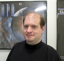
Now moving into a Phase II study funded by NASA’s Innovative Advanced Concepts office (NIAC), the idea is dubbed Thin-Film Nuclear Engine Rocket (TFINER). Not the world’s most pronounceable acronym, but if the idea works out, that will hardly matter. Working at the Charles Stark Draper Laboratory, a non-profit research and development company in Cambridge MA, Bickford is known to long-time Centauri Dreams readers for his work on naturally occurring antimatter capture in planetary magnetic fields. See Antimatter Acquisition: Harvesting in Space for more on this.

Image: Draper Laboratory’s Jim Bickford, taking a deep space propulsion concept to the next level. Credit: Charles Stark Draper Laboratory.

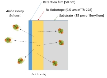
Harvesting naturally occurring antimatter in space offers some hope of easing one of the biggest problems of such propulsion strategies, namely the difficulty in producing enough antimatter to fuel an engine. With the Thin Film Nuclear Engine Rocket, Bickford again tries to change the game. The notion is to use energetic radioisotopes in thin layers, allowing their natural decay products to propel a spacecraft. The proper substrate, Bickford believes, can control the emission direction, and the sail-like system packs a punch: Velocity changes on the order of 100 kilometers per second using mere kilograms of fuel.

I began this piece talking about ‘Oumuamua, but that’s just for starters. Because if we can create a reliable propulsion system capable of such tantalizing speed. we can start thinking about mission targets as distant as the solar gravitational focus, where extreme magnifications become possible. Because the lensing effect for practical purposes begins at 550 AU and continues with a focal line to infinity, we are looking at a long journey. Bear in mind that Voyager 1, our most distant working spacecraft, has taken almost half a century to reach, as of now, 167 AU. To image more than one planet at the solar lens, we’ll also need a high degree of maneuverability to shift to multiple exoplanetary systems.

Image: This is Figure 3-1 from the Phase 1 report. Caption: Concept for the thin film thrust sheet engine. Alpha particles are selectively emitted in one direction at approximately 5% of the speed of light. Credit: NASA/James Bickford.

So we’re looking at a highly desirable technology if TFINER can be made to work, one that could offer imaging of exoplanets, outer planet probes, and encounters with future interstellar interlopers. Bickford’s Phase 1 work will be extended in the new study to refine the mission design, which will include thruster experiments as well as what the Phase II summary refers to as ‘isotope production paths’ while also considering opportunities for hybrid missions that could include the Oberth ‘solar dive’ maneuver. More on that last item soon, because Bickford will be presenting a paper on the prospect this summer.

Image: Artist concept highlighting the novel approach proposed by the 2025 NIAC awarded selection of the TFINER concept. This is the baseline TFINER configuration used in the system analysis. Credit: NASA/James Bickford.

But let’s drop back to the Phase I study. I’ve been perusing Bickford’s final report. Developing out of Wolfgang Moeckel’s work at NASA Lewis in the 1970s, the TFINER design uses thin sheets of radioactive elements. The solution leverages exhaust velocities for alpha particle decays that can exceed 5 percent of the speed of light. You’ll recall my comment on space sails in the previous post, where we looked at the advantage of inflatable components to make sails more scalable. TFINER is more scalable still, with changes to the amount of fuel and sheet area being key variables.

Let’s begin with a ~10-micron thick Thorium-228 radioisotope film, with each sheet containing three layers, integrating the active radioisotope fuel layer in the middle. Let me quote from the Phase I report on this:

It must be relatively thin to avoid substantial energy losses as the alpha particles exit the sheet. A thin retention film is placed over this to ensure that the residual atoms do not boil off from the structure. Finally, a substrate is added to selectively absorb alpha emission in the forward direction. Since decay processes have no directionality, the substrate absorber produces the differential mass flow and resulting thrust by restricting alpha particle trajectories to one direction.

The TFINER baseline uses 400 meter tethers to connect the payload module. The sheet’s power comes from Thorium-228 decay (alpha decay) — the half-life is 1.9 years. We get a ‘decay cascade chain’ that produces daughter products – four additional alpha emissions result with half-lives ranging from 300 ns to 3 days. The uni-directional thrust is produced thanks to the beryllium absorber (~35-microns thick) that coats one side of the thin film to capture emissions moving forward. Effective thrust is thus channeled out the back.

Note as well the tethers in the illustration, necessary to protect the sensor array and communications component to minimize the radiation dose. Manipulation of the tethers can control trajectory on single-stage missions to deep space targets. Reconfiguring the thrust sheet is what makes the design maneuverable, allowing thrust vectoring, even as longer half-life isotopes can be deployed in the ‘staged’ concept to achieve maximum velocities for extended missions.

Image: This is Figure 7-8 from the report. Caption: Example thrust sheet rotation using tether control. Credit: NASA/James Bickford.

From the Phase I report:

The payload module is connected to the thrust sheet by long tethers. A winch on the payload module can individually pull-in or let-out line to manipulate the sail angle relative to the payload. The thrust sheet angle will rotate the mean thrust vector and operate much like trimming the sail of a boat. Of course, in this case, the sail (sheet) pressure comes from the nuclear exhaust rather than the wind

It’s hard to imagine the degree of maneuverability here being replicated in any existing propulsion strategy, a big payoff if we can learn how to control it:

This approach allows the thrust vector to be rotated relative to the center of mass and velocity vector to steer the spacecraft’s main propulsion system. However, this is likely to require very complex controls especially if the payload orientation also needs to be modified. The maneuvers would all be slow given the long lines lengths and separations involved.

Spacecraft pointing and control is an area as critical as the propulsion system. The Phase I report goes into the above options as well as thrust vectoring through sheets configured as panels that could be folded and adjusted. The report also notes that thermo-electrics within the substrate may be used to generate electrical power, although a radioisotope thermal generator integrated with the payload may prove a better solution. The report offers a good roadmap for the design refinement of TFINER coming in Phase II.

Inflatable Technologies for Deep Space

One idea for deep space probes that resurfaces every few years is the inflatable sail. We’ve seen keen interest especially since Breakthrough Starshot’s emergence in 2016 in meter-class sails, perhaps as small as four meters to the side. But if we choose to work with larger designs, sails don’t scale well. Increase sail area and problems of mass arise thanks to the necessary cables between sail and payload. An inflatable beryllium sail filled with a low-pressure gas like hydrogen avoids this problem, with payload mounted on the space-facing surface. Such sails have already been analyzed in the literature (see below).

Roman Kezerashvili (City University of New York), in fact, recently analyzed an inflatable torus-shaped sail with a twist, one that uses compounds incorporated into the sail material itself as a ‘propulsive shell’ that can take advantage of desorption produced by a microwave beam or a close pass of the Sun. Laser beaming also produces this propulsive effect but microwaves are preferable because they do not damage the sail material. Kezerashvili has analyzed carbon in the sail lattice in solar flyby scenarios. The sail is conceived as “a thin reflective membrane attached to an inflatable torus-shaped rim.”

Image: This is Figure 1 from the paper. Credit: Kezerashvili et al.

Inflatable sails go back to the late 1980s. Joerg Strobl published a paper on the concept in the Journal of the British Interplanetary Society, and it received swift follow-up in a series of studies in the 1990s examining an inflatable radio telescope called Quasat. A series of meetings involving Alenia Spazio, an Italian aerospace company based in Turin, took the idea further. In 2018, Claudio Maccone, Greg Matloff, and NASA’s Les Johnson joined Kezerashvili in analyzing inflatable technologies for missions as challenging as a probe to the Oort Cloud.

Indeed, working with Joseph Meany in 2023, Matloff would also describe an inflatable sail using aerograpahite and graphene, enabling higher payload mass and envisioning a ‘sundiver’ trajectory to accelerate an Alpha Centauri mission. The conception here is for a true interstellar ark carrying a crew of several hundred, using a sail with radius of 764 kilometers on a 1300 year journey. So the examination of inflatable sails in varying materials is clearly not slowing down.

The Inflatable Starshade

But there are uses for inflatable space structures that go beyond outer system missions. I see that they are now the subject of a NIAC Phase I study by John Mather (NASA GSFC) that puts a new wrinkle into the concept. Mather’s interest is not propulsion but an inflatable starshade that, in various configurations, could work either with the planned Habitable Worlds Observatory or an Extremely Large Telescope like the 39 m diameter European Extremely Large Telescope now being built in Chile. Starshades are an alternative to coronagraph technologies that suppress light from a star to reveal its planetary companions.

Inflatables may well be candidates for any kind of large space structure. Current planning on the Habitable Worlds Observatory, scheduled for launch no earlier than the late 2030s, includes a coronagraph, but Mather thinks the two technologies offer useful synergies. Here’s a quote from the study summary:

A starshade mission could still become necessary if: A. The HWO and its coronagraph cannot be built and tested as required; B. The HWO must observe exoplanets at UV wavelengths, or a 6 m HWO is not large enough to observe the desired targets; C. HWO does not achieve adequate performance after launch, and planned servicing and instrument replacement cannot be implemented; D. HWO observations show us that interesting exoplanets are rare, distant, or are hidden by thick dust clouds around the host star, or cannot be fully characterized by an upgraded HWO; or E. HWO observations show that the next step requires UV data, or a much larger telescope, beyond the capability of conceivable HWO coronagraph upgrades.

So Mather’s idea is also meant to be a kind of insurance policy. It’s worth pointing out that coronagraphs are well studied and compact, while starshade technologies are theoretically sound but untested in space. But as the summary mentions, work at ultraviolet wavelengths is out of the coronagraph’s range. To get into that part of the spectrum, pairing Habitable Worlds Observatory with a 35-meter starshade seems the only option. This conceivably would allow a relaxation of some HWO optical specs, and thus lower the overall cost. The NIAC study will explore these options for a 35-meter as well as a 60-meter starshade.

I mentioned the possibility of combining a starshade with observations through an Extremely Large Telescope, an eye-widening notion that Mather proposed in a 2022 NIAC Phase I study. The idea here is to place the starshade in an orbit that would match position and velocity with the telescope, occulting the star to render the planets more visible. This would demand an active propulsion system to maintain alignment during the observation, while also making use of the adaptive optics already built into the telescope to suppress atmospheric distortion. The mission is called Hybrid Observatory for Earth-like Exoplanets.

Image: Artist concept highlighting the novel approach proposed by the 2025 NIAC awarded selection of Inflatable Starshade for Earthlike Exoplanets concept. Credit: NASA/John Mather.

As discussed earlier, mass considerations play into inflatable designs. In the HOEE study, Mather referred to his plan “to cut the starshade mass by more than a factor of 10. There is no reason to require thousands of kg to support 400 kg of thin membranes.” His design goal is to create a starshade that can be assembled in space, thus avoiding launch and deployment issues. All this to create what he calls “the most powerful exoplanet observatory yet proposed.”

You can see how the inflatable starshade idea grows out of the hybrid observatory study. By experimenting with designs producing the needed strength, stiffness, stability and thermal requirements and the issues raised by bonding large sheets of materials of the requisite strength, the mass goals may be realized. So the inflatable sail option once again morphs into a related design, one optimized as an adjunct to an exoplanet observatory, provided this early work can lead to a solution that could benefit both astronomy and sails.

The paper on inflatable beryllium sails is Matloff, G. L., Kezerashvili, R. Ya., Maccone, C. and Johnson, L., “The Beryllium Hollow-Body Solar Sail: Exploration of the Sun’s Gravitational Focus and the Inner Oort Cloud”, arXiv:0809.3535v1 [physics.space-ph] 20 Sep 2008. The later Kezerashvili paper is Kezerashvili et al., “A torus-shaped solar sail accelerated via thermal desorption of coating,” Advances in Space Research Vol. 67, Issue 9 (2021), pp. 2577-2588 (abstract). The Matloff and Meany paper on an Alpha Centauri interstellar ark is ”Aerographite: A Candidate Material for Interstellar Photon Sailing,” JBIS Vol. 77 (2024) pp. 142-146. Thanks to Thomas Mazanec and Antonio Tavani for the pointer to Mather’s most recent NIAC study.

Odd Couple: Gas Giants and Red Dwarfs

The assumption that gas giant planets are unlikely around red dwarf stars is reasonable enough. A star perhaps 20 percent the mass of the Sun should have a smaller protoplanetary disk, meaning sufficient gas and dust to build a Jupiter-class world are lacking. The core accretion model (a gradual accumulation of material from the disk) is severely challenged. Moreover, these small stars are active in their extended youth, sending out frequent flares and strong stellar winds that should dissipate such a disk quickly. Gravitational instabilities within the disk are one possible alternative.

Planet formation around such a star must be swift indeed, which accounts for estimates as low as 1 percent of such stars having a gas giant in the system. Exceptions like GJ 3512 b, discovered in 2019, do occur, and each is valuable. Here we have a giant planet, discovered through radial velocity methods, orbiting a star a scant 12 percent of the Sun’s mass. Or consider the star GJ 876, which has two gas giants, or the exoplanet TOI-5205 b, a transiting gas giant discovered in 2023. Such systems leave us hoping for more examples to begin to understand the planet forming process in such a difficult environment.

Let me drop back briefly to a provocative study from 2020 by way of putting all this in context before we look at another such system that has just been discovered. In this earlier work, the data were gathered at the Atacama Large Millimeter/submillimeter Array (ALMA), taken at a wavelength of 0.87 millimeters. The team led by Nicolas Kurtovic (Max Planck Institute for Astronomy, Heidelberg) found evidence of ring-like structures in protoplanetary disks that extend between 50 and 90 AU out.

Image: This is a portion of Figure 2 from the paper, which I’m including because I doubt most of us have seen images of a red dwarf planetary disk. Caption: Visibility modeling versus observations of our sample. From left to right: (1) Real part of the visibilities after centering and deprojecting the data versus the best fit model of the continuum data, (2) continuum emission of our sources where the scale bar represents a 10 au distance, (3) model image, (4) residual map (observations minus model), (5) and normalized, azimuthally averaged radial profile calculated from the beam convolved images in comparison with the model without convolution (purple solid line) and after convolution (red solid line). In the right most plots, the gray scale shows the beam major axis. Credit: Kurtovic et al.

Gaps in these rings, possibly caused by planetary embryos, would accommodate planets of the Saturn class, and the researchers find that gaps formed around three of the M-dwarfs in the study. The team suggests that ‘gas pressure bumps’ develop to slow the inward migration of the disk, allowing such giant worlds to coalesce. It’s an interesting possibility, but we’re still early in the process of untangling how this works. For more, see How Common Are Giant Planets around Red Dwarfs?, a 2021 entry in these pages.

Now we learn of TOI-6894 b, a transiting gas giant found as part of Edward Bryant’s search for such worlds at the University of Warwick and the University of Liège. An international team of astronomers confirmed the find using telescopes at the SPECULOOS and TRAPPIST projects. The work appears in Nature Astronomy (citation below). Here’s Bryant on the scope of the search for giant M-dwarf planets:

“I originally searched through TESS observations of more than 91,000 low-mass red-dwarf stars looking for giant planets. Then, using observations taken with one of the world’s largest telescopes, ESO’s VLT, I discovered TOI-6894 b, a giant planet transiting the lowest mass star known to date to host such a planet. We did not expect planets like TOI-6894b to be able to form around stars this low-mass. This discovery will be a cornerstone for understanding the extremes of giant planet formation.”

TOI-6894 b has a radius only a little larger than Saturn, although it has only about half of Saturn’s mass. What adds spice to this particular find is that the host star is the lowest mass star found to have a transiting giant planet. In fact, TOI-6894 is only 60 percent the size of the next smallest red dwarf with a transiting gas giant. Given that 80 percent of stars in the Milky Way are red dwarfs, determining an accurate percentage of red dwarf gas giants is significant for assessing the total number in the galaxy.

Image: Artwork depicting the exoplanet TOI-6894 b around a red dwarf star. This planet is unusual because, given the size/mass of the planet relative to the very low mass of the star, this planet should not have been able to form. The planet is vary large compared to its parent star, shown here to scale. With the known temperature of the star, the planet is expected to only be approximately 420 degrees Kelvin at the top of its atmosphere. This means its atmosphere may contain methane and ammonia, amongst other species. This would make this planet one of the first planets outside the Solar System where we can observe nitrogen, which alongside carbon and oxygen is a key building block for life. Credit: University of Warwick / Mark Garlick.

TOI-6894 b produces deep transits and sports temperatures in the range of 420 K, according to the study. Clearly this world is not in the ‘hot Jupiter’ category. Amaury Triaud (University of Birmingham) is a co-author on this paper:

“Based on the stellar irradiation of TOI-6894 b, we expect the atmosphere is dominated by methane chemistry, which is exceedingly rare to identify. Temperatures are low enough that atmospheric observations could even show us ammonia, which would be the first time it is found in an exoplanet atmosphere. TOI-6894 b likely presents a benchmark exoplanet for the study of methane-dominated atmospheres and the best ‘laboratory’ to study a planetary atmosphere containing carbon, nitrogen, and oxygen outside the Solar System.”

Thus it’s good to know that JWST observations targeting the atmosphere of this world are already on the calendar within the next 12 months. Rare worlds that can serve as benchmarks for hitherto unexplained processes are pure gold for our investigation of where and how giant planets form.

The paper is Bryant et al., “A transiting giant planet in orbit around a 0.2-solar-mass host star,” Nature Astronomy (2025). Full text. The Kurtovic study is Kurtovic, Pinilla, et al., “Size and Structures of Disks around Very Low Mass Stars in the Taurus Star-Forming Region,” Astronomy & Astrophysics, 645, A139 (2021). Full text.

Expansion of the Universe: An End to the ‘Hubble Tension’?

When one set of data fails to agree with another over the same phenomenon, things can get interesting. It’s in such inconsistencies that interesting new discoveries are sometimes made, and when the inconsistency involves the expansion of the universe, there are plenty of reasons to resolve the problem. Lately the speed of the expansion has been at issue given the discrepancy between measurements of the cosmic microwave background and estimates based on Type Ia supernovae. The result: The so-called Hubble Tension.

It’s worth recalling that it was a century ago that Edwin Hubble measured extragalactic distances by using Cepheid variables in the galaxy NGC 6822. The measurements were necessarily rough because they were complicated by everything from interstellar dust effects to lack of the necessary resolution, so that the Hubble constant was not known to better than a factor of 2. Refinements in instruments tightened up the constant considerably as work progressed over the decades, but the question of how well astronomers had overcome the conflict with the microwave background results remained.

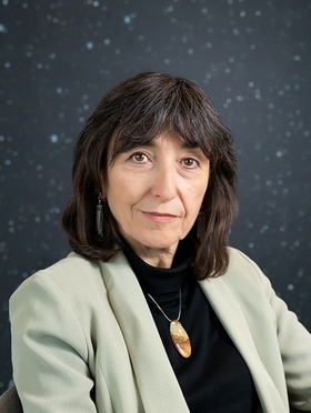
Now we have new work that looks at the rate of expansion using data from the James Webb Space Telescope, doubling the sample of galaxies used to calibrate the supernovae results. The paper’s lead author, Wendy Freedman of the University of Chicago, argues that the JWST results resolve the tension. With Hubble data included in the analysis as well, Freedman calculates a Hubble value of 70.4 kilometers per second per megaparsec, plus or minus 3%. This result brings the supernovae results into statistical agreement with recent cosmic microwave background data showing 67.4, plus or minus 0.7%.

Image: The University of Chicago’s Freedman, a key player in the ongoing debate over the value of the Hubble Constant. Credit: University of Chicago.

While the cosmic microwave background tells us about conditions early in the universe’s expansion, Freedman’s work on supernovae is aimed at pinning down how fast the universe is expanding in the present, which demands accurate measurements of interstellar distances. Knowing the maximum brightness of supernovae allows the use of their apparent luminosities to calculate their distance. Type 1a supernovae are consistent in brightness at their peak, making them, like the Cepheid variables Hubble used, helpful ‘standard candles.’

The same factors that plagued Hubble, such as the effect of dimming from interstellar dust and other factors that affect luminosity, have to be accounted for, but JWST has four times the resolution of the Hubble Space Telescope, and is roughly 10 times as sensitive, making its measurements a new gold standard. Co-author Taylor Hoyt (Lawrence Berkeley Laboratory) notes the result:

“We’re really seeing how fantastic the James Webb Space Telescope is for accurately measuring distances to galaxies. Using its infrared detectors, we can see through dust that has historically plagued accurate measurement of distances, and we can measure with much greater accuracy the brightnesses of stars.”

Image: Scientists have made a new calculation of the speed at which the universe is expanding, using the data taken by the powerful new James Webb Space Telescope on multiple galaxies. Above, Webb’s image of one such galaxy, known as NGC 1365. Credit: NASA, ESA, CSA, Janice Lee (NOIRLab), Alyssa Pagan (STScI).

A lack of agreement between the CMB findings and the supernovae data could have been pointing to interesting new physics, but according to this work, the Standard Model of the universe holds up. In a way, that’s too bad for using the discrepancy to probe into mysterious phenomena like dark energy and dark matter, but it seems we’ll have to be looking elsewhere for answers to their origin. Ahead for Freedman and team are new measurements of the Coma cluster that Freedman suggests could fully resolve the matter within years.

As the paper notes:

While our results show consistency with ΛCDM (the Standard Model), continued improvement to the local distance scale is essential for further reducing both systematic and statistical uncertainties.

The paper is Freedman et al., “Status Report on the Chicago-Carnegie Hubble Program (CCHP): Measurement of the Hubble Constant Using the Hubble and James Webb Space Telescopes,” The Astrophysical Journal Vol. 985, No 2 (27 May 2025), 203 (full text).

Megastructures: Adrift in the Temporal Sea

Here about the beach I wander’d, nourishing a youth sublime
With the fairy tales of science, and the long result of Time…

—Tennyson

Temporal coincidence plays havoc with our ideas about other civilizations in the cosmos. If we want to detect them, their society must at least have developed to the point that it can manipulate electromagnetic waves. But its technology has to be of sufficient strength to be noticed. The kind of signals people were listening to 100 years ago on crystal sets wouldn’t remotely fit the bill, and neither would our primitive TV signals of the 1950s. So we’re looking for strong signals and cultures older than our own.

Now consider how short a time we’re talking about. We have been using radio for a bit over a century, which is on the order of one part in 100,000,000 of the lifespan of our star. You may recall the work of Brian Lacki, which I wrote about four years ago (see Alpha Centauri and the Search for Technosignatures). Lacki, now at Oxford, points out how unlikely it would be to find any two stars remotely near each other whose civilization ‘window’ corresponded to our own. In other words, even if we last a million years as a technological civilization, we’re just the blink of an eye in cosmic time.

Image: Brian Lacki, whose work for Breakthrough Listen continues to explore both the scientific and philosophical implications of SETI. Credit: University of Oxford.

Adam Frank at the University of Rochester has worked this same landscape. He thinks we might well find ourselves in a galaxy that at one time or another had flourishing civilizations that are long gone. We are separated not only in space but also in time. Maybe there are such things as civilizations that are immortal, but it seems more likely that all cultures eventually end, even if by morphing into some other form.

What would a billion year old civilization look like? Obviously we have no idea, but it’s conceivable that such a culture, surely non-biological and perhaps non-corporeal, would be able to manipulate matter and spacetime in ways that might simply mimic nature itself. Impossible to find that one. A more likely SETI catch would be a civilization that has had space technologies just long enough to have the capability of interstellar flight on a large scale. In a new paper, Lacki looks at what its technosignature might look like. If you’re thinking Dyson spheres or swarms, you’re on the right track, but as it turns out, such energy gathering structures have time problems of their own.

Lacki’s description of a megaswarm surrounding a star:

These swarms, practically by definition, need to have a large number of elements, whether their purpose is communication or exploitation. Moreover, the swarm orbital belts need to have a wide range of inclinations. This ensures that the luminosity is being collected or modulated in all directions. But this in turn implies a wide range of velocities, comparable to the circular orbital velocity. Another problem is that the number of belts that can “fit” into a swarm without crossing is limited.

Image: Artist’s impression of a Dyson swarm. Credit: Archibald Tuttle / Wikimedia Commons. CC BY-SA 4.0.

Shards of Time

The temporal problem persists, for even a million year ‘window’ is a sliver on the cosmic scale. The L factor in the Drake equation is a great unknown, but it is conceivable that the death of a million-year old culture would be survived by its artifacts, acting to give us clues to its past just as fossils tell us about the early stages of life on Earth. So might we hope to find an ancient, abandoned Dyson swarm around a star close enough to observe?

Lacki is interested in failure modes, the problem of things that break down. Helpfully, megastructures are by definition gigantic, and it is not inconceivable that. Dyson structures of one kind or another could register in our astronomical data. As the paper notes, a wide variety covering different fractions of the host star can be imagined. We can scale a Dyson swarm down or up in size, with perhaps the largest ever proposed being from none other than Nikolai Kardashev, who discusses in a 1985 paper a disk parsecs-wide built around a galactic nucleus (!).

I’m talking about Dyson swarms instead of spheres because from what we know of material science, solid structures would suffer from extreme instabilities. But swarms can be actively managed. We have a history of interest in swarms dating back to 1958, when Project Needles at MIT contemplated placing a ring of 480,000,000 copper dipole antennas in orbit to enhance military communications (the idea was also known as Project West Ford). Although two launches were carried out experimentally, the project was eventually shelved because of advances in communications satellites.

So we humans already ponder enclosing the planet in one way or another, and planetary swarms, as Lacki notes, are already with us, considering the constellations of satellites in Earth orbit, the very early stages of a mini Dyson swarm. Just yesterday, the announcement by SpinLaunch that it will launch hundreds of microsatellites into orbit using a centrifugal cannon gave us another instance. Enclosing a star in a gradually thickening swarm seems like one way to harvest energy, but if such structures were built, they would have to be continuously maintained. The civilization behind a Dyson swarm needs to survive if the swarm itself is to remain viable.

For the gist of Lacki’s paper is that on the timescales we’re talking about, an abandoned Dyson swarm would be in trouble within a surprisingly short period of time. Indeed, collisions can begin once the guidance systems in place begin to fail. What Lacki calls the ‘collisional time’ is roughly an orbital period divided by the covering fraction of the swarm. How long it takes to develop into a ‘collisional cascade’ depends upon the configuration of the swarm. Let me quote the paper, which identifies:

…a major threat to megastructure lifespans: if abandoned, the individual elements eventually start crashing into each other at high speeds (as noted in Lacki 2016; Sallmen et al. 2019; Lacki 2020). Not only do the collisions destroy the crashed swarm members, but they spray out many pieces of wreckage. Each of these pieces is itself moving at high speeds, so that even pieces much smaller than the original elements can destroy them. Thus, each collision can produce hundreds of missiles, resulting in a rapid growth of the potentially dangerous population and accelerating the rate of collisions. The result is a collisional cascade, where the swarm elements are smashed into fragments, that are in turn smashed into smaller pieces, and so on, until the entire structure has been reduced to dust. Collisional cascades are thought to have shaped the evolution of minor Solar System body objects like asteroid families and the irregular satellites of the giant planets (Kessler 1981; Nesvorn.

You might think that swarm elements could be organized so that their orbits reduce or eliminate collisions or render them slow enough to be harmless. But gravitational perturbations remain a key problem because the swarm isn’t an isolated system, and in the absence of active maintenance, its degradation is relatively swift.

Image: This is Figure 2 from the paper. Caption: A sketch of a series of coplanar belts heating up with randomized velocities. In panel (a), the belt is a single orbit on which elements are placed in an orderly fashion. Very small random velocities (meters per second or less) cause small deviations in the elements’ orbits, though so small that the belt is still “sharp”, narrower than the elements themselves (b). The random velocities cause the phases to desynchronize, leading to collisions, although they are too slow to damage the elements (cyan bursts). The collision time decreases rapidly in this regime until the belt is as wide as the elements themselves and becomes “fuzzy” (c). The collision time is at its minimum, although impacts are still too small to cause damage. In panel (d), the belts are still not wide enough to overlap, but relative speeds within the belts have become fast enough to catastrophically damage elements (yellow explosions), and are much more frequent than the naive collisional time implies because of the high density within belts. Further heating causes the density to fall and collisions to become rarer until the belts start to overlap (e). Finally, the belts grow so wide that each belt overlaps several others, with collisions occuring between objects in different belts too (f), at which point the swarm is largely randomized. Credit: Brian Lacki.

Keeping the Swarm Alive

Lacki’s mathematical treatment of swarm breakdown is exhaustive and well above my payscale, so I send you to the paper if you want to track the calculations that drive his simulations. But let’s talk about the implications of his work. Far from being static technosignatures, megaswarms surrounding stars are shown to be highly vulnerable. Even the minimal occulter swarm he envisions turns out to have a collision time of less than a million years. A megaswarm needs active maintenance – in our own system, Jupiter’s gravitational effect on a megaswarm would destroy it within several hundred thousand years. These are wafer-thin time windows if scaled against stellar lifetimes.

The solution is to actively maintain the megaswarm and remove perturbing objects by ejecting them from the system. An interesting science fiction scenario indeed, in which extraterrestrials might sacrifice systems planet by planet to maintain a swarm. Lacki works the simulations through gravitational perturbations from passing stars and in-system planets and points to the Lidov-Kozai effect, which turns circular orbits at high inclination into eccentric orbits at low inclination. Also considered is radiation pressure from the host star and radiative forces resulting from the Yarkovsky effect.

How else to keep a swarm going? From the paper:

For all we know, the builders are necessarily long-lived and can maintain an active watch over the elements and actively prevent collisions, or at least counter perturbations. Conceivably, they could also launch tender robots to do the job for them, or the swarm elements have automated guidance. Admittedly, their systems would have to be kept up for millions of years, vastly outlasting anything we have built, but this might be more plausible if we imagine that they are self-replicating. In this view, whenever an element is destroyed, the fragments are consumed and forged into a new element; control systems are constantly regenerated as new generations of tenders are born. Even then, self-replication, repair, and waste collection are probably not perfectly efficient.

The outer reaches of a stellar system would be a better place for a Dyson swarm than the inner system, which would be hostile to small swarm elements, even though the advantage of such a position would be more efficient energy collection. The habitable zone around a star is perhaps the least likely place to look for such a swarm given the perturbing effects of other planets. And if we take the really big picture, we can talk about where in the galaxy swarms might be likely: Low density environments where interactions with other stars are unlikely, as in the outskirts of large galaxies and in their haloes. “This suggests,” Lacki adds, “that megaswarms are more likely to be found in regions that are sometimes considered disfavorable for habitability.”

Ultimately, an abandoned Dyson swarm is ground into microscopie particles via the collision cascades Lacki describes, evolving into nothing more than dispersed ionized gas. If we hope to find an abandoned megastructure like this in our practice of galactic archaeology, what are the odds that we will find it within the window of time within which it can survive without active maintenance? We’d better hope that the swarm creators have extremely long-lived civilizations if we are to exist in the same temporal window as the swarm we want to observe. A dearth of Dyson structures thus far observed may simply be a lack of temporal coincidence, as we search for systems that are inevitably wearing down without the restoring hand of their creators.

The paper is Lacki, “Ground to Dust: Collisional Cascades and the Fate of Kardashev II Megaswarms,” accepted at The Astrophysical Journal (preprint). The Kardashev paper referenced above is “On the Inevitability and the Possible Structure of Super Civilizations,” in The Search for Extraterrestrial Life: Recent Developments, ed. M. D. Papagiannis, Vol. 112, 497–504.

The Statistically Quantitative Information from Null Detections of Living Worlds: Lack of positive detections is not a fruitless search

It’s no surprise, human nature being what it is, that our early detections of possible life on other worlds through ‘biosignatures’ are immediately controversial. We have to separate signs of biology from processes that may operate completely outside of our conception of life, abiotic ways to produce the same results. My suspicion is that this situation will persist for decades, claim vs. counter-claim, with heated conference sessions and warring papers. But as Alex Tolley explains in today’s essay, even a null result can be valuable. Alex takes us into the realm of Bayesian statistics, where prior beliefs are gradually adjusted as new data come in. We’re still dealing with probabilities, but in a fascinating way, uncertainties are gradually being decreased though never eliminated. We’re going to be hearing a lot more about these analytical tools as the hunt continues with next generation telescopes.

by Alex Tolley

Introduction

The venerable Drake equation’s early parameters are increasingly constrained as our exoplanet observations continue. We now have a good sample of thousands of exoplanets to estimate the fraction of planets in the habitable zone that could support life. This last firms up the term ne, the mean number of planets that could support life per star with planets.

This is now a shift to focus on the fraction of habitable planets with life (fl). The first to confirm a planet with life will likely make the history books.

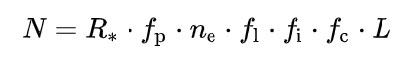
However, as with the failure of SETI to receive a signal from extraterrestrial intelligence (ETI) since the 1960s, there will be disappointments in detecting extraterrestrial life. The early expectation of Martian vegetation proved incorrect, as did the controversial Martian microbes thought to have been detected by the Viking lander life detection experiments in 1976. More recently, the phosphine biosignature in the Venusian atmosphere has not been confirmed, and now the claimed dimethyl sulfide (DMS) biosignature on K2-18b is also questioned.

While we hope that an unambiguous biosignature is detected, are null results just disappointments that have no value in determining whether life is present in the cosmos, or do they add some value in determining a frequency of habitable planets with life?

Before diving into a recent paper that attempts to answer this question, I want to give a quick introduction to statistics. The most common type of statistics is Fisher statistics, where collected sample data is used to calculate the distribution parameters for the population from which the sample is taken. This approach is used when the sample size is greater than 1 or 2, and is most often deployed in calculating the accuracy of a mean value and 95% range of values as part of a test of significance. This approach works well when the sample contains sufficient examples to represent the population. For binary events, such as heads in a coin test, the Binomial distribution will provide the expected frequencies of unbiased and small biases in coin tosses.

However, a problem arises when the frequency of a binary event is extremely low, so that the sample of events detects no positive events, such as heads, at all. In the pharmaceutical industry, while efficacy of a new drug needs a large sample size for validity, the much larger phase 4 marketing period is used to monitor for rare side effects that are not discoverable in the clinical trials. There have been a number of well known drugs that were withdrawn from the market during this period, perhaps the most famous being thalidomide and its effects on fetal development. In such circumstances, Fisherian statistics are unhelpful in determining probabilities of rare events with sample sizes inadequate to catch these rare events. As we have seen with SETI, the lack of any detected signal provides no value for the probability that ETI exists, only that it is either rare, or that ETI is not signaling. All SETI scientists can do is keep searching with the hope that eventually a signal will be detected.

Bayesian statistics are a different approach that can help overcome the problem of determining the probability of rare events, one that has gained in popularity over the last few decades. It assumes a prior belief, perhaps no more than a guess, of the probability of an event, and then adjusts it with new observed data as they are acquired. For example, one assumes a coin toss is 50:50 heads or tails. If the succeeding tosses show only tails, then the coin toss is biased, and each new resulting tail decreases the probability of a head resulting on the next toss. For our astrobiological example, if life is very infrequent on habitable worlds, Bayesian statistics can be informative to estimate the probability of detection success.

In essence, the Bayesian method updates beliefs in the probability of events, given the new observations of the event. With a large enough number of observations, the true probability of an event value will emerge that will either converge or diverge from the initial expected probability.

I hope it is clear that this Bayesian approach is well-suited to the announcement of detecting a biosignature on a planet, where detections to date have either been absent or controversial. Each detection or lack of detection in a survey will update our expectations of the frequency of life. At this time, the probability of life on a potentially habitable planet ranges from 0 (life is unique to Earth) to 1.0 (some form of life appears wherever it is possible) Beliefs that the abiogenesis of life is extremely hard due to its complexity push the probability of life being detected as close to 0. Conversely, the increasing evidence that life emerges quickly on a new planet, such as within 100 million years on Earth [6], implies that the probability of a habitable planet having life is close to 1.0.

The Angerhausen et al paper I am looking at today (citation below) considers a number of probability distributions depending on beliefs about the probability of life, rather than a single value for each belief. These are shown in Figure 1 and explained in Box 2. I would in particular note the Kerman and Jeffreys distributions that are bimodal with the highest likelihoods for the distributions as the extremes, and reflect the “fine tuning” argument for life by Kipping et al [2] explained in the Centauri Dreams post [3] i.e., either life will be almost absent, or ubiquitous, and not some intermediate probability of appearing on a habitable planet, In other words, the probability is either very close to 0 or close to 1.0, but unlikely to be some intermediate probability. The paper relies on the Beta function [Box 3] that uses the probability of positive and negative events defined by 2 parameters for the binary state of the event, e.g. life detected or not detected. This function can approximate the Binomial distribution, but can handle the different probability distributions.

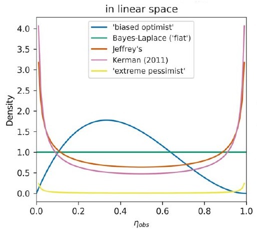
Figure 1. The five different prior distributions as probability density functions (PDF) used in the paper and explained in Box 2. Note the Kerman and Jeffreys distributions that bias the probabilities at the extremes, compared to the “biased optimist” that has 3 habitable worlds around the sun (Venus, Earth, and Mars), but with only the Earth having life.

The Beta function is adjusted by the number of observations or positive and negative detections of biosignatures. At this point, the positive and negative observations are based on the believed prior distributions which can take any values, from guesses to preliminary observational results, which at this time are relatively few. After all, we are still arguing over whether we have even detected biosignature molecules, let alone confirmed their detection. We then adjust those expectations by the new observations.

What happens when we start a survey and gain events of biosignature detection? Using the Jeffreys prior distribution, let us see the effect of observing no biosignature detections for up to 100 negative biosignature observations.

Figure 2a. The effect of increasing the null observations on a skewed distribution that shows the increasing certainty of the low probability frequencies. While apparently the high probabilities also rise, the increase in null detections implies that the relative frequency of positives declines.

Figure 2b. The increasing certainty that the frequency of life on habitable planets tends towards 0 as the number of null biosignature detections increases. The starting value of 0.5 is taken from the Jeffreys prior distribution. The implied frequency is the new frequency of positives as the null detections reduce the frequency observed and push the PDF towards the lower bound of 0 (see figure 1)

So far, so good. If we can be sure that the biosignature detection is unambiguous and that the inference that life is present or absent can be inferred with certainty based on the observations, then the sampling of up to 100 habitable worlds will indicate whether life is rare or ubiquitous and can be determined with high confidence. If every star system had at least 1 habitable world, this sample would include most stars within 20 ly of Earth. In reality, if we limit our stars to spectral types F, G & K, which represent 5-10% of all stars, and half of these have at least 1 habitable world, then we need to search 2000-4000 star systems, which are well within 100 ly, a tiny fraction of the galaxy.

The informed reader should now balk at the status of this analysis. Biosignatures are not unambiguous [4]. Firstly, detecting a faint trace of a presumed biosignature gas is not certain, as the phosphine on Venus and the DMS/DMDS on TOI-270d detections make clear. They are both controversial. In the case of Venus, we are neither certain that the phosphine signal is present and that the correct identification has been made, nor that there is no abiogenic mechanism to create phosphine in Venus’ very different environment. As discussed in my post on the ambiguity of biosignatures, prior assumptions about biosignatures as unambiguous were reexamined, with the response that astrobiologists built a scale of certainties for assessing whether a planet is inhabited based on the contextual interpretation of biosignature data.[4].

The authors of the paper allow for this by modifying the formula to allow for both false-positive and false-negative biosignature detection rates, and also for interpretation uncertainty of the detected biosignature. The authors also calculate the upper bound at about 3 sigma (99.9%) of the frequency of observations. Figure 3 shows the effect of these uncertainties on the location and size of the maximal probability density function for the Jeffrey’s Bayesian priors.

Figure 3. The effects of sample and interpretation, best fit, and 99.9% uncertainties for null detections. As both sample and interpretation uncertainty increase, the expected number of positive detections increases. The Jeffrey prior’s distribution is used.

Figure 3 implies that with interpretation uncertainty of just 10%, even 100 null observations, the calculated frequency of life increases 2 orders of magnitude from 0.1% to 10%. The upper bound increases from less than 10% to between 20 and 30%. Therefore, even if 100 new observations of habitable planets with no detected biosignatures, the frequency of inhabited planets is between ⅕ and ⅓ of habitable planets at this level of certainty. As one can see from the asymptotes, no amount of further observations will increase the certainty that life is absent in the population of stars in the galaxy. Uncertainty is the gift that allows astrobiologists to maintain hope that there are living worlds to discover.

Lastly, the authors apply their methodology to 2 projects to discover habitable worlds; the Habitable Worlds Observatory [7] and the Large Interferometer for Exoplanets (LIFE} concepts. The analyses are shown in figure 4. The vertical lines indicate the expected number of positive detections by the conceptual methods and the expected frequencies of detections with their associated upper bounds due to uncertainty.

Figure 4. Given the uncertainties, the authors calculate the 99.9% ( > 3 sigma) upper limit on the null hypothesis of no life and matched against data obtained by 2 surveys by Morgan with The Habitable Worlds Observatory (HWO) and 2 by Kammerer with The Large Interferometer for Exoplanets (LIFE) [7, 8].

The authors note that it may be incorrect to use the term “habitable” if water is detected, or “living” if a biosignature[s] is detected. They suggest it would be better to just use the calculation for the detection method, rather than the implication of the detection, that is, that the sample uncertainty, but not the interpretation uncertainty, is calculated. As we see in the popular press, if a planet in the habitable zone (HZ) has about an Earth-size mass and density, this planet is sometimes referred to as “Earth 2.0” with all the implications of the comparison to our planet. However, we know that our current global biosphere and climate are relatively recent in Earth’s history. The Earth has experienced different states from anoxic atmosphere, to extremely hot, and conversely extremely cold periods in the past. It is even possible the world may be a dry desert, like Venus, or conversely a hycean world with no land for terrestrial organisms to evolve.

However, even if life and intelligence prove rare and very sparsely distributed, a single, unambiguous signature, whether of a living world or a signal with information, is detected, the authors state:

Last but not least we want to remind the reader here that, even if this paper is about null results, a single positive detection would be a watershed moment in humankind’s history.

In summary, Bayesian analysis of null detections against prior expectations of frequencies can provide some estimate of the upper limit frequency of living worlds, with many null detections reducing the frequencies and their upper limits. Using Fisherian statistics, many null detections would provide no such estimates, as all the data values would be 0 (null detections). The statistics would be uninformative other than that as the number of null detections increased, the expectation of the frequency of living worlds would qualitatively decrease.

While planetologists and astrobiologists would hope that they would observationally detect habitable and inhabited exoplanets, as the uncertainties are decreased and the number of observations continues to show null results, how long before such activities become a fringe, uneconomic activity that results in lost opportunity costs for other uses of expensive telescope time?

The paper is Angerhausen, D., Balbi, A., Kovačević, A. B., Garvin, E. O., & Quanz, S. P. (2025). “What if we Find Nothing? Bayesian Analysis of the Statistical Information of Null Results in Future Exoplanet Habitability and Biosignature Surveys”. The Astronomical Journal, 169(5), 238. https://doi.org/10.3847/1538-3881/adb96d

References

1. Wikipedia “Drake equation” https://en.wikipedia.org/wiki/Drake_equation. Accessed 04/12/2025

2. Kipping & Lewis, “Do SETI Optimists Have a Fine-Tuning Problem?” submitted to International Journal of Astrobiology (preprint). https://arxiv.org/abs/2407.07097

3. Gilster P. “The Odds on an Empty Cosmos“ Centauri Dreams, Aug 16, 2024 https://www.centauri-dreams.org/2024/08/16/the-odds-on-an-empty-cosmos/

4. Tolley A. “The Ambiguity of Exoplanet Biosignatures“ Centauri Dreams Jun 21, 2024
https://www.centauri-dreams.org/2024/06/21/the-ambiguity-of-exoplanet-biosignatures/

5. Foote, Searra, Walker, Sara, et al. “False Positives and the Challenge of Testing the Alien Hypothesis.” Astrobiology, vol. 23, no. 11, Nov. 2023, pp. 1189–201. https://doi.org/10.1089/ast.2023.0005.

6. Tolley, A. Our Earliest Ancestor Appeared Soon After Earth Formed. Centauri Dreams, Aug 28, 2024 https://www.centauri-dreams.org/2024/08/28/our-earliest-ancestor-appeared-soon-after-earth-formed/

7. Wikipedia “Habitable Worlds Observatory” https://en.wikipedia.org/wiki/Habitable_Worlds_Observatory. Accessed 05/02/2025

8. Kammerer, J. et al (2022) “Large Interferometer For Exoplanets (LIFE) – VI. Detecting rocky exoplanets in the habitable zones of Sun-like stars. A&A, 668 (2022) A52
DOI: https://doi.org/10.1051/0004-6361/202243846