Ivan Idris's Blog, page 17

NumPy Cookbook chapter 5

Chapter 5 of NumPy Cookbook is about audio and image processing. The contents of chapter 5 of NumPy Cookbook:

Loading images in memory maps
Adding images
Blurring images
Repeating audio fragments
Generating sounds
Designing an audio filter
Edge detection with the Sobel filter




The book [...]

NumPy Cookbook chapter 4

Chapter 4 of NumPy Cookbook is about NumPy interoperability features and NumPy on the Cloud. The preliminary contents of chapter 4 of NumPy Cookbook:

Using the buffer protocol
Using the array interface
Exchanging data with Matlab and Octave
Installing RPy2
Interfacing with R
Installing JPype
Sending a [...]

NumPy Cookbook chapter 3

Chapter 3 of NumPy Cookbook is about commonly used functions. The preliminary contents of chapter 3 of NumPy Cookbook:

Summing Fibonacci numbers
Finding Prime Factors
Finding Palindromic numbers
Steady State Vector determination
Discovering a power law
Sieving Integers with the Sieve of Erasthothenes

The book is due [...]

NumPy Cookbook Chapter 2

Chapter 2 of NumPy Cookbook is entitled “Advanced indexing and array concepts”. The preliminary contents of chapter 2 of NumPy Cookbook:

Install SciPy
Install PIL
Install Matplotlib
Slice multidimensional arrays of images
Indexing with booleans
Indexing with lists of indices
Select rows and columns with the ix [...]

NumPy Cookbook Chapter 1

Chapter 1 of NumPy Cookbook is about IPython. The preliminary contents of chapter 1 of NumPy Cookbook:

Installing IPython
Using IPython as a shell
Reading manual pages
Configuring IPython
Running a HTML notebook
Exporting a HTML notebook
Importing a HTML notebook
Running a public notebook server

The book is [...]

Imminent Release of NumPy Cookbook

After a long hiatus I am back to announce the imminent release of NumPy Cookbook. NumPy cookbook is in many ways meant as a follow-up of NumPy 1.5 Beginner’s Guide and is targeted at more experienced NumPy users. The release [...]

Statistical Bootstrapping by Case Resampling

NumPy Strategies 0.1.7
I haven’t blogged in a while, because I am supposed to work on a Big Secret Project (BSP). Obviously, I am not allowed to talk about that. The Product Owner/Manager of our FHF (Fantasy Hedge Funds) has come [...]

Simulated Random Trading

NumPy Strategies 0.1.6
Our Product Owner and Product Manager got talking about our latest strategy. They decided that our Fantasy Hedge Fund needs to have simulations of these strategies. The new User Story:

Simulate periodic trading with random buying and selling.

We will [...]

NumPy Project Euler Problem 9

Project Euler Problem 9 is a tough one. After reading the Pythagorean Triple Wikipedia page, I implemented a NumPy solution with Euclid's Formula.




1. Create m and n arrays
The Euclid's Formula defines indices m and n. We will create arrays to [...]

NumPy Periodic Dips

NumPy Strategies 0.1.5

The stock market has periodic dips to the downside and sometimes to the upside, but those have a different name. Our Fantasy Hedge Fund needs to rebalance its portfolio 5 times a year (this is all part of our plan of Total World Domination). Therefore this User Story:

I want to buy and sell stocks 5 times a year.

We will have a look at the probability distribution of the stock price log returns.

1. Get close prices

Let's start by downloading historical data for a stock. For instance, AAPL.

1
2
3
4
5
today = date.today()
start = (today.year - 1, today.month, today.day)
 
quotes = quotes_historical_yahoo(sys.argv[1], start, today)
close = numpy.array([q[4] for q in quotes])

2. Get log returns

Second, calculate the daily log returns of the close prices.

1
logreturns = numpy.diff(numpy.log(close))

3. Calculate breakout and pullback

Now comes the interesting part. Let's say we want to trade 5 times per year or roughly every 50 days. One strategy would be to buy when the price drops by a certain percentage and sell when the price increases by another percentage. By setting the percentile appropriate for our trading frequency, we can match the corresponding log returns. Scipy offers the scoreatpercentile function, that we will use.

1
2
3
freq = 1/float(sys.argv[2])
breakout = scipy.stats.scoreatpercentile(logreturns, 100 * (1 - freq) )
pullback = scipy.stats.scoreatpercentile(logreturns, 100 * freq)

4. Generate buys and sells

Use the NumPy compress function to generate buys and sells for our close price data.

1
2
3
4
5
6
buys = numpy.compress(logreturns < pullback, close)
sells = numpy.compress(logreturns > breakout, close)
print buys
print sells
print len(buys), len(sells)
print sells.sum() - buys.sum()

The output for AAPL and a 50 day period is:

1
2
3
4
[ 340.1 377.35 378. 373.17 415.99]
[ 357. 370.8 366.48 395.2 419.55]
5 5
24.42

So we have a profit of 24 dollar, if we buy and sell 5 times an AAPL share.

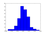
5. Plot a histogram of the log returns

Just for fun let's plot the histogram of the log returns with Matplotlib.

1
2
matplotlib.pyplot.hist(logreturns)
matplotlib.pyplot.show()

Below is the complete code or get it from Github.

1
2
3
4
5
6
7
8
9
10
11
12
13
14
15
16
17
18
19
20
21
22
23
24
25
26
27
28
29
30
31
32
33
from matplotlib.finance import quotes_historical_yahoo
from datetime import date
import numpy
import sys
import scipy.stats
import matplotlib.pyplot
 
#1. Get close prices.
today = date.today()
start = (today.year - 1, today.month, today.day)
 
quotes = quotes_historical_yahoo(sys.argv[1], start, today)
close = numpy.array([q[4] for q in quotes])
 
#2. Get log returns.
logreturns = numpy.diff(numpy.log(close))
 
#3. Calculate breakout and pullback
freq = 1/float(sys.argv[2])
breakout = scipy.stats.scoreatpercentile(logreturns, 100 * (1 - freq) )
pullback = scipy.stats.scoreatpercentile(logreturns, 100 * freq)
 
#4. Generate buys and sells
buys = numpy.compress(logreturns < pullback, close)
sells = numpy.compress(logreturns > breakout, close)
print buys
print sells
print len(buys), len(sells)
print sells.sum() - buys.sum()
 
#5. Plot a histogram of the log returns
matplotlib.pyplot.hist(logreturns)
matplotlib.pyplot.show()

If you liked this post and are interested in NumPy check out NumPy Beginner's Guide by yours truly.