Paul Gilster's Blog, page 55

TRAPPIST-1: Seven Worlds of Similar Compostion

Image: Artist’s depiction of the TRAPPIST-1 star and its seven worlds. Credit: NASA/JPL-Caltech/R. Hurt (IPAC).

As if we needed another indication that the TRAPPIST-1 system is utterly different from our own, consider new work led by Eric Agol (University of Washington), which examines this seven-planet system in terms of the planets’ density. The planets here are all similar in size to Earth. Compare that with the huge range in planetary size we see in our own system. The new work tightens orbital dynamics and calculates their densities, showing they are all about 8 percent less dense than the rocky planets around Sol.

In the paper, the TRAPPIST-1 densities are calculated through analysis of abundant data (over 1,000 hours of observation by Spitzer alone, along with significant contributions from Kepler and ground-based telescopes like TRAPPIST and SPECULOOS). They are refined through computer simulations on planetary orbits, showing a system where planetary composition begs for an explanation.

We’re dealing with a system under intense scrutiny, one about which we have ever-tightening parameters on planetary diameter, mass and density, so we have much to work with. The work pauses briefly to consider a possible eighth planet:

Our mass precisions are predicated on a complete model of the dynamics of the system. We ignore tides and general relativity, which are too small in amplitude to affect our results at the current survey duration and timing precision (Bolmont et al. 2020). Should an eighth planet be lurking at longer orbital periods, which has yet to reveal itself via significant TTVs or transits, this may modify our timing solution and shift the masses slightly. In our timing search for an additional planet, however, we found that such a planet might only cause shifts at the ≈1σ level.

Agol worked with colleagues Zachary Langford and Victoria Meadows at the University of Washington, and an international team including scientists based in Switzerland, France, the UK and Morocco. Says Agol:

“This is one of the most precise characterizations of a set of rocky exoplanets, which gave us high-confidence measurements of their diameters, densities and masses. This is the information we needed to make hypotheses about their composition and understand how these planets differ from the rocky planets in our solar system.”

[image error]

Image: Shown here are three possible interiors of the TRAPPIST-1 exoplanets. The more precisely scientists know the density of a planet, the more they can narrow down the range of possible interiors for that planet. All seven planets have very similar densities, so they likely have a similar compositions. Credit: NASA/JPL-Caltech.

The researchers examine the TRAPPIST-1 planets in terms of the proportion of iron, oxygen, magnesium and silicon thought to make up rocky worlds in any system. The 8 percent difference in density is explicable through several competing hypotheses.

A lower percentage of iron — 21 percent as compared to Earth’s 32 percent — would do the trick, possibly indicating a core with a lower relative mass (most of Earth’s iron is found in its core). Alternatively, planets enriched with oxygen compared to the Earth could produce iron oxide — rust — in abundance, possibly extending to the core (Earth, Mars, Mercury and Venus have cores of unoxidized iron). A combination of both these scenarios is possible, according to Agol, with the TRAPPIST-1 planets having less iron than our system’s rocky worlds but with a larger amount of it being oxidized.

A third possibility is that these planets are enriched with water compared to the Earth. Surfaces covered with water would change a planet’s overall density. This would demand amounts of water totalling 5 percent of the total mass of the four outer planets (by comparison, water makes up less than 0.1 percent of the Earth’s total mass). This would also imply hot, dense atmospheres for the three inner worlds at TRAPPIST-1.

Each hypothesis has consequences in terms of planet formation. Water worlds imply origins beyond the snow line, an environment rich in ice, with the planets subsequently migrating inward toward the host star. Long-term planetary configurations can form from migration, and the stability of TRAPPIST-1’s system has been examined in earlier work. Tightening up the constraints on planetary mass and orbital eccentricity allows the authors to again consider the question. They find that the idea of migration also fits the hypothesis of a fully oxidized planetary core. From the paper:

…the lower measured bulk densities of the TRAPPIST-1 planets relative to Earth-like composition might be explained by core-free interiors (Elkins-Tanton & Seager 2008) in which the oxygen content is high enough such that all iron is oxidized. If the refractory elements (Mg, Fe, Si) follow solar abundances, a fully oxidized interior would contain about 38.2 wt% of oxygen, which lies between the value for Earth (29.7 wt%) and CI chondrites (45.9 wt%). Such an interior scenario can easily describe the observed bulk densities…, and this may bolster the long-range migration scenario in which the planets formed in a highly oxidizing environment that enabled the iron to remain in the mantle even after migration.

One thing that would drive this work further is more information about the composition of the M8 red dwarf that hosts the planetary system. The authors point out that measurements of the Mg/Fe and Fe/Si ratios would affect the interpretation of their results on planetary cores and mantle composition.

And as we see so often in such work, a functioning James Webb Space Telescope is pointed to as a possibility for producing even more precise constraints on system dynamics and planetary bulk densities, which would aid in choosing among the competing hypotheses for composition. For all of this, the TRAPPIST-1 system is an ideal testing ground, as co-author Caroline Dorn (University of Zurich) notes:

“The night sky is full of planets, and it is only within the last 30 years that we have been able to begin to unravel their mysteries. The TRAPPIST-1 system is fascinating because around this unique star we can learn about the diversity of rocky planets within a single system. And we can also learn more about a planet by studying its neighbours, so this system is perfect for that.”

The paper is Agol et al., “Refining the Transit-timing and Photometric Analysis of TRAPPIST-1: Masses, Radii, Densities, Dynamics, and Ephemerides,” Planetary Science Journal Vol. 2, No. 1 (22 January 2021). Full text.

Was the Wow! Signal Due to Power Beaming Leakage?

The Wow! signal has a storied history in the SETI community, a one-off detection at the Ohio State ‘Big Ear’ observatory in 1977 that Jim Benford, among others, considers the most interesting candidate signal ever received. A plasma physicist and CEO of Microwave Sciences, Benford returns to Centauri Dreams today with a closer look at the signal and its striking characteristics, which admit to a variety of explanations, though only one that the author believes fits all the parameters. A second reception of the Wow! might tell us a great deal, but is such an event likely? So far all repeat observations have failed and, as Benford points out, there may be reason to assume they must. The essay below is a shorter version of the paper Jim has submitted to Astrobiology.

by James Benford

In 1977 the Big Ear radio telescope (Ohio State University Radio Telescope) recorded the famous Wow! Signal, which is the most serious contender for artificial interstellar radiation. It is called the ‘Wow!’ Signal. It has never been seen again. Its origin and nature remain a total mystery.

I offer an alternative explanation for it: The Wow! could have been leakage from an interstellar power beam. I propose that this class of radiation, which is not widely understood, can explain the observed features of the Wow! signal.

The Three Wow! Parameters

The Wow! signal has 3 prominent parameters: the power density received, the signal’s duration and its frequency [1].

Power Density: The Wow! signal was very strong, the strongest they ever recorded in the seven-year Ohio State SETI Survey. The shape is shown in the Figure.

Figure: The Wow! Signal. The peak is 32 times the signal to noise ratio of the observations. Courtesy of Sam Morrell.

Duration: The Big Ear was fixed in orientation, so rotated with the Earth. From Gray [1]: “The amount of time it took the Wow! to pass through the antenna’s beam closely matches the expected transit time for celestial sources. Sources fixed amid the stars should take about 36 seconds to transit the sensitive middle half of the beam, the full-width-half-max. The Wow! signal took about 38 seconds”.

So we don’t know how long the signal lasted, just that it was on as the antenna rotated past.

Frequency: The Wow! Signal was at 1.42 GHz. The 1.4-1.427 GHz band is protected internationally, meaning, as John Kraus, designer and director at the Big Ear, says in a letter to Carl Sagan , “all emissions are prohibited” [2]. The band was set aside to allow radio astronomy of the H 1 line, the hyperfine transition of neutral hydrogen (1.420 GHz), which is of great astronomical interest for imaging atomic hydrogen in interstellar space. Consequently, this part of the L-band is a protected radio astronomy allocation all over the world. Therefore the Wow! couldn’t be a transmission from Earth satellites or aircraft.

The Fourth Wow! Parameter

There is a fourth parameter, although it has not received attention: the Revisit Time. This is the interval until the signal is seen again. If ET were rastering their beam across the sky, the beam would be seen to repeat later. Searches have been conducted from the META array at Oak Ridge, the Green Bank National Radio Astronomy Observatory in West Virginia and the Tasmanian Mount Pleasant Radio Observatory in Australia [3, 4].

Recent extensive observations on the Allen Array by Gerry Harp, Robert Gray and colleagues, which used the 42 dishes of the ATA as an interferometer, monitored the entire 1.5 degree field of view for 100 hours. They did not see the Wow! and summarized [5]: “As for the possibility that the Wow! signal is a repetitive transient, our observations rule out almost all periods under 40 hours, which covers many repetitive scenarios such as rotating planets or blinking beacons with periods comparable to a terrestrial day and several times longer. Our extended observations cannot rule out scenarios such as occasional targeted transmissions with repetition rates of many days or varying repetition rates.”

The Wow! observation has never recurred. I take this absence as a clue to its origin.

Power Beaming and the Wow! Signal

The most observable leakage radiation from an advanced civilization may well be from the use of power beaming to accelerate spacecraft and transfer energy. Power beams are now more credible because we’re building our own: The Starshot project plans launching probes to nearby stars in this century, making power beaming a credible source concept [6]. And power beaming is being developed for military applications, where it is termed ‘directed energy’ [7]. See reference 8 for a review of power beaming concept studies.

Applications suggested for power beaming are:

launching spacecraft to orbit,raising satellites to a higher orbit,interplanetary space–to–space transfers of cargo or passengers,beam-driven launch of interstellar probes,beam-driven starships.

Leakage of the beam around the sides of the vehicle being accelerated would be observable at great range because of the highly directed high power. The spilled energy can be reduced to less than half, but that is not the cost optimum. Spillage losses of more than half are typical of Starshot calculations, for reasons of economics and performance that will apply to other civilizations [6].

For power beam missions involving changing orbits of spacecraft, the first three applications on the above list, an important quantity is the slew rate, the rate at which the beam propelling the spacecraft sweeps to direct it toward its orbit [8]. A review of representative parameters for applications of power beaming shows that, for orbit–related missions, the slew rates are high, so the observation time of the beam leakage is too short, ≲ 1 second. So the orbit–related applications cannot explain the Wow! But interstellar probes and starships have small slew rate, so are the best candidates.

Power Beaming Examples

In beaming of power, the power density S at range R is determined by W, the effective isotropic radiated power (EIRP), which is the product of radiated peak power P and aperture gain G [8]. Since we know the power density of the Wow! received and its frequency, we can calculate both the range to the source of Wow! and the power needed at a given range.

For example, if the Wow! source had the EIRP of Arecibo, it would have to be at range < 2 light-years, so it must be far more powerful.

Bob Forward’s ultralight microwave-propelled Starwisp, a 1-kg sail reaching 0.1 c, would be at a range of ~ a million light-years, so from extra-galactic distances [9].

An interstellar precursor probe described by Benford and Matloff for 100 km/sec = 0.03% c would be at range 116 light-years, a nearby star [10].

We can also assume a distance, then calculate the EIRP that would be required. First, choose 2000 light-years for the distance to the Wow! source. (Maccone estimates that the mean distance to a communicative civilization is ~2,000 light-years away [11]). Then choose an aperture diameter of 3 km. (Starshot envisions a ~3-km diameter laser array to drive its interstellar probe.) The required beam power is 11 GW. This is similar to Starshot, with ~ 11 GW.

From these examples, it is credible that the Wow! signal was leakage from launch of an interstellar probe.

Will we see it again? Probably not

Probably not if it was due to power beaming. With a launch driven by an intense beam, to arrive years later at a neighboring stellar system, the starship would be launched toward where the stellar system will be when the starship arrives. The ratio of the distance the star would move to the beam spot size is given by vs/(vss Δθ), where vs is the average velocity of the star relative to stars on our stellar neighborhood, typically 20 km/sec, and vss is the starship velocity, Δθ the angular beamwidth. For the starship concepts proposed, that ratio varies from 104 to 107 [8].

The angle of the radiated beam with respect to the light path between the two stars is larger than the width of the beam. Thus, the beam is generally not observable from the target planetary system. If the Wow! was driving a probe to a star, that star was at that time far from the direction of the beam. Earth could accidentally receive the leakage from the beam, since stars move relative to each other. So leakage radiation from star probe launches using the Wow! beam will not be seen again from Earth. This fits the non-observations to date.

Comparison of Explanations for the Wow! Signal

There are three suggested explanations for the Wow!: either spurious emissions from Earth, an interstellar communication or leakage from a power beam. Here is a brief summary of the evidence for and against each explanation:

Arguments for power beaming leakage as a cause:

The power beaming explanation for the Wow! accounts for all four of the Wow! parameters: the power density received, the duration of the signal, its frequency, and the reason why the Wow! has not occurred again. The Wow! power beam leakage hypothesis gets stronger the longer that listening for the Wow! to recur doesn’t observe it repeat.Power beams are now more credible because we’re building our own: the Starshot project plans launching probes to nearby stars in this century. The technology required for the Beamers for such interstellar probe launches are within our grasp.

Arguments against ET communication as a cause:

The theory that the Wow! Signal was an interstellar communication predicts that it will recur. It fits within the overall SETI strategy, which looks for deliberate beaming of messages to us from ETI. But the long series of the subsequent non-observations of the Wow! shows that the SETI messaging hypothesis is gradually being falsified by being tested.

Arguments against radio frequency interference (RFI) as a cause:

The Wow! Signal was at 1.42 GHz. The band from 1.4 to 1.427 GHz is protected internationally, meaning, all emissions are prohibited [2]. Therefore it is very doubtful that the Wow! Was a transmission from Earth satellites or aircraft because they are forbidden to transmit in this band. Secret satellites would avoid it because they would be detected by radio astronomers. (Emissions in this band are sometimes detected, but at very low levels. These are likely due to intermodulation products, which are nonlinear effects in electronics.)Aircraft would be unlikely to remain static in the sky. Spacecraft would pass through the beam much faster. To match that lack of angular motion, an Earth satellite would have to be millions of kilometers distant, out far beyond the Moon.Ohio had good RFI rejection because what was recorded was the difference between two offset beams, so a local signal appearing in both horns simultaneously would cancel. This was frequently verified.The possibility that the signal was a harmonic or sub-harmonic of a local signal is countered by Ohio State having monitored the 21 cm band for many years, would have noticed a local interfering signal.A deliberate hoax? This lacks credibility, as hoaxes are a practical joke, which succeed if they are later revealed. Then why keep it secret for decades?Conclusion and Implications

I’ve looked at the various power beaming applications and found that credible ones are low mass interstellar probes such as Starwisp and Starshot. This does not mean that the orbit–changing power-beaming applications cannot be seen.

The power beaming explanation for the Wow! accounts for all four of the Wow! parameters. This includes the absence of any later observation, for it has not been seen since, despite the several attempts to repeat observing it. This allows a prediction: the Wow! signal will not be seen again.

If one accepts the possibility that Wow! was power beam leakage, several lines of action should be followed for the future of SETI:

Such interstellar power beams would be visible over large interstellar distances. All-sky surveys in both the microwave and laser could detect more power beam leakages. Instruments with large instantaneous field of view could detect infrequent transitory leakage signals. Ultimately, we should have a full-sky capability for both hemispheres.Because ET would understand that its beam leakage could be observed, there may well be modulations on the beam to communicate to any inadvertent listener. This would add little additional energy or cost for ET. Therefore all-sky surveys should have sufficient electronics to capture messaging embedded on the beam. Extraterrestrial intelligences would know their power beams could be observed. That message may use optimized power-efficient designs such as spread spectrum and energy minimization [12, 13].

On the other hand, if one thinks that the Wow! signal was an attempt to communicate, one should follow up on a possibility that is not been explored: If with Wow! we inadvertently intercepted a radio link between one star and another, we should look in the opposite direction to see if signals are transmitting toward the Wow! direction. To my knowledge this has not been explored.

References

1. R. H. Gray, The Elusive Wow!, Palmer Square Press, 2012.

2. J. D. Kraus, “The Tantalizing “Wow!” Signal”, letter to Carl Sagan, NRAO Archives, accessed December 3, 2020, https://www.nrao.edu/archives/items/show/3684, 1994.

3. R. H. Gray, “Intermittent Signals and Planetary Days in SETI”, Int. J. Astrobiology, https://doi.org/10.1017/S1473550420000038

4. R. H. Gray, A Search For Periodic Emissions At The Wow! Locale”, Astrophysical Journal, 578:967–971, 2002.

5. G. Harp et al., “An ATA Search for a Repetition of the Wow! Signal”, Astrophysical Journal 160:162, 2020.

6. K. Parkin, “The Breakthrough Starshot System Model”, Acta Astronautica 152, 370, 2018.

7. J. Benford, J. Swegle and E. Schamiloglu, High Power Microwaves, 3rd Ed., Taylor & Francis, Boca Raton, FL 2016.

8. J. Benford and D. Benford, “Power Beaming Leakage Radiation as a SETI Observable”, Astrophysical Journal 101 825, 2016.

9. R. L. Forward, “Starwisp: An Ultralight Interstellar Probe,” J. Spacecraft and Rockets, 22 345-350 1985.

10. J. Benford and G. Matloff, Intermediate Beamers for Starshot”, JBIS 72, 51, 2019.

11. C. Maccone, “The Statistical Drake Equation”, Acta Astronautica 67, 1366, 2010.

12. D. Messerschmitt, “The case for spread spectrum”, Acta Astronautica, 81, 227, 2012.

13. D. Messerschmitt, 2015, ‘Design for minimum energy in interstellar communication”, Acta Astronautica, 107, 20-39, 2015.

Propulsion for Satellite ‘Constellations’

A French company called Exotrail has been working on electric propulsion systems for small spacecraft down to the CubeSat level. As presented last week at the 13th European Space Conference in Brussels, the ExoMG Hall-effect electric propulsion system was flown in a demonstration orbital mission in November, launched to low-Earth orbit by a PSLV (Polar Satellite Launch Vehicle) rocket. A brief nod to the PSLV: These launch vehicles were developed by the Indian Space Research Organisation (ISRO), and are being used for rideshare launch services for small satellites. Among their most notable payloads have been the Indian lunar probe Chandrayaan-1, and the Mars Orbiter Mission called Mangalyaan.

Hall-effect thrusters (HET) trap electrons emitted by a cathode in a magnetic field, ionizing a propellant to create a plasma that can be accelerated via an electric field. The technology has been in use in large satellites for many years because of its high thrust-to-power ratio.

What catches my eye about ExoMG is its size, about that of a 2-liter bottle of soda as opposed to conventional Hall-effect thrusters that weigh in at refrigerator size and demand kilowatts of power. The Exotrail thruster, which was successfully fired during the November mission, runs on about 50 watts of power, and appears to be a propulsion system that can adapt to satellites in the range of 10 to 250 kg. Collision avoidance and deorbiting for satellites in the CubeSat range as well as flexible orbital operations become feasible with this technology.

Image: Satellite using Exotrail technology undergoing testing. Credit: Exotrail.

The company is calling ExoMG “the first ever Hall-effect thruster operating on a sub-100kg spacecraft,” and points to four missions slated to fly with the technology in 2021. I’m interested in how the diminutive thruster can be employed in constellations of satellites. We already rely on satellites working together as a system — GPS is a classic example. The needs of navigation and communication force the issue. Think Iridium and Globalstar in terms of telephony, or the Russian Molniya military and communications satellites. The list could be easily extended.

So what we have evolving is a set of constellation technologies with immediate application to satellites in low-Earth orbit. Exotrail talks about “high coverage telecommunication constellations or high revisit rate earth observation constellations at 600-2000km altitude,” enabled by orbit-raising via the new thrusters as well as necessary de-orbiting capabilities, but we should be looking as well at the controlling software and thinking in longer timeframes. Satellites working together is the theme.

Increasing miniaturization coupled with artificial intelligence and next-generation electric thrusters can be enablers for planetary probes flying in swarm formation in the outer system, perhaps using sail technologies as the primary propulsion to get them there. The one-size fits all purposes mission begins to give way to a fleet approach, tiny probes networking their data as they operate at targets as interesting as Neptune and Pluto. It’s also worth noting that the entire Breakthrough Starshot concept calls for not one but an armada of small sails in interstellar space, offering a hedge against catastrophic failure of any one craft, and conceivably drawing on swarm technologies that could facilitate data gathering and return.

So I keep an eye on near-term technologies that explore this space of miniaturization, efficient orbital adjustment and constellation operations. It will be intriguing to see how Exotrail’s operational software (called ExoOPS) deals with the interactions of such constellations. Likewise interesting is last fall’s firing of the European Space Agency’s Helicon Plasma Thruster, which ESA presents as a “compact, electrodeless and low voltage design” optimized for propulsion in small satellites, including “maintaining the formation of large orbital constellations.”

The HPT achieved its first test ignition back in 2015 at ESA’s Propulsion Laboratory in the Netherlands, and has been under development in terms of improved levels of ionization and acceleration efficiency ever since, using high-power radio frequency waves, as opposed to the application of an electrical current, to render propellant into a plasma for acceleration.

Image: A test firing of Europe’s Helicon Plasma Thruster, developed with ESA by SENER and the Universidad Carlos III’s Plasma & Space Propulsion Team (EP2-UC3M) in Spain. This compact, electrodeless and low voltage design is ideal for the propulsion of small satellites, including maintaining the formation of large orbital constellations. Credit: SENER.

Where will constellation and formation flying in Earth orbit take us as we adapt them for environments further out? Will we one day see deep space swarms of Cubesat-sized (and smaller) craft exploring the outer planets?

TOI-1259A: Implications of a White Dwarf Companion

TESS, our Transiting Exoplanet Survey Satellite, continues to roll up interesting planet candidates, with over 2450 TESS Objects of Interest (TOI) thus far identified. The one that catches my eye this morning showed up in the lightcurve of TOI-1259A, a K-dwarf some 385 light years away. The planet designated TOI-1259Ab is Jupiter-sized but some 56 percent less massive, with a 3.48 day orbit at 0.04 AU, and an equilibrium temperature of 963 K.

This system gets interesting, though, not so much for the planet but the other star, a white dwarf (TOI-1259B) in a wide orbit at 1648 AU from the K-dwarf. A team of astronomers led by David Martin (Ohio State University) finds an effective temperature of 6300 K, a radius of 0.013 solar radii and a mass of 0.56 solar masses, a set of characteristics that allow the team to estimate that the system is just over 4 billion years old.

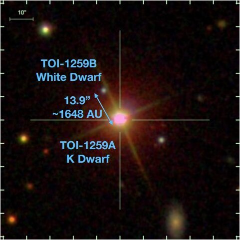
Image: SDSS image of the planet host TOI-1259A and its bound white dwarf companion TOI-1259B. Credit: Martin et al., 2021.

Let’s home in on the issue of white dwarfs, for they force a significant question: How does the evolution of a star affect the evolution of the planetary system around it? The system containing TOI-1259Ab may prove useful in helping us understand the processes at work.

But first, what about white dwarfs themselves? A star like the Sun will expand into a red giant perhaps five billion years from now, ultimately leaving a white dwarf remnant, with whatever planetary survivors still intact left transformed by the process.

So it’s not surprising that about 50 percent of the white dwarfs studied show atmospheres polluted by heavy elements. That would be an indication of material from the surrounding system accreting onto the white dwarf. Still noteworthy, though, is the fact that you would expect such heavy elements to settle out in the presence of the white dwarf’s high gravity. The process of accretion must, then, be relatively common, allowing the stellar atmosphere to be constantly replenished.

White dwarfs produce their own set of challenges when it comes to exoplanet discovery. Finding planets around them is relatively rare. From the paper on the TOI-1259Ab work, I learned that these stars show a lack of the kind of sharp spectral features that would allow precise characterization using radial velocity methods. The push and pull of orbiting worlds is less evident than it would be around other classes of star.

That seems to throw us back on transit methods, something both Kepler and TESS turned into an art, but here we’re dealing with the problem that white dwarfs have a small radius. They’re roughly the size of the Earth, which means that transit probabilities are reduced and so are transit durations. Moreover, according to Martin et al., white dwarfs are faint enough that their light curves are noisy, a problem for astrometric methods — think Gaia — as well.

So while we’ve found atmospheric pollutants at these stars, and have tagged transits of planetary debris, the first confirmed planet orbiting a white dwarf wasn’t found until recently (for more on WD 1856+534, see On White Dwarf Planets as Biosignature Targets).

But back to TOI-1259Ab, which is not a white dwarf planet, but a tightly orbiting Jupiter-sized planet around a K-dwarf. Here the white dwarf is a distant but definitely bound second star. It turns out that even systems with planets and white dwarf companions are rare, as the paper notes:

Only a few bona fide planets have been discovered with degenerate outer companions (Table 2), the first being Gliese-86b (Queloz et al. 2000; Els et al. 2001; Lagrange et al. 2006). Mugrauer (2019) found 204 binary companions in a sample of roughly 1300 exoplanet hosts, of which eight of the companions were white dwarfs. Mugrauer & Michel (2020) found five white dwarf companions to TESS Objects of Interest, including TOI-1259, but without radial velocity data to confirm the TOIs as planets. Some of these planets were also in the El-Badry & Rix (2018) catalogue.

Stellar systems that include white dwarfs have much to teach us, and in the case of TOI-1259Ab, we have a world that has now been confirmed through radial velocity follow-up, and a white dwarf that influenced it. Driving this research forward will be the question of how systems with a degenerate outer companion object evolve, for there are implications here for planetary dynamics. This system should be an interesting target for the James Webb Space Telescope. Consider: The transit depth is 2.7 percent on the K-dwarf host star, which is 0.71 percent of the Sun’s radius. Moreover, its location places the system near the TESS and JWST continuous viewing zones.

The authors believe that the white dwarf in this system is far enough from the K-dwarf that it would not affect the formation of planets, but go on to point out that while it was on the main sequence, it progenitor star would have been both more massive and also closer, which would have made it a factor in orbital dynamics for TOI-1259Ab. The planet’s tight orbit may thus be at least partially the result of migration forced by the now degenerate white dwarf companion.

On the matter of stellar age, it’s worth noting that white dwarfs cool steadily as they age, which helps astronomers constrain the age of the star and the system around it using its temperature and luminosity. Let me quote the paper on this, because star age is so tricky to determine for other stellar types:

If the WD’s mass is known, the initial mass of its progenitor star can be inferred through the initial-final mass relation (IFMR), and this initial mass constrains the pre-WD age of the WD progenitor. Therefore if we have a well-constrained distance to the WD then its total age, i.e. the sum of its main sequence lifetime and its cooling age, can be robustly measured from its spectral energy distribution (SED). Under the reasonable ansatz that the WD and K dwarf formed at the same time, we can then measure the total system age from the WD.

Another useful insight offered by white dwarfs, the study of which may help us explain unusual system architectures like this one, as well as informing us on outcomes as stars and their companions are transformed over time.

The paper is Martin et al., “TOI-1259Ab – a gas giant planet with 2.7% deep transits and a bound white dwarf companion,” submitted to Monthly Notices of the Royal Astronomical Society (preprint).

Recovering a Triple Star Planet with New Data

The Kepler mission produced so much data — 2394 exoplanets, 2366 candidates by the end of spacecraft operations in 2018 — that we might forget how quickly all this came about. The first Kepler results started being announced in 2010. One of these, the second candidate to emerge, was KOI-5Ab, which was a tough pick in the early going given its position within a triple star system. An ambiguous detection, it was soon left behind, its status uncertain, as the numbers of more definitive candidates swelled. Caltech’s David Ciardi, who discussed this elusive system at the recent virtual meeting of the American Astronomical Society, says this about it:

“KOI-5Ab got abandoned because it was complicated, and we had thousands of candidates. There were easier pickings than KOI-5Ab, and we were learning something new from Kepler every day, so that KOI-5 was mostly forgotten.”

Ciardi, who is chief scientist at NASA’s Exoplanet Science Institute, has now pulled KOI-5Ab back to vibrant life. Almost certainly a gas giant, the planet orbits one of three stars in the system in a misaligned orbit that calls into question the nature of its formation. Making original confirmation of the planet difficult was the inability to completely distinguish it from the possible effects of the other two stars in the system. Untangling the question would involve TESS data. The object appears in TESS terminology as TOI-1241b, showing a five-day orbit that matches the Kepler result.

Confirming such a candidate calls for more than a single backup asset on the ground. Working with colleagues in the California Planet Search, Ciardi used Keck data, as well as observations from Caltech’s Palomar Observatory near San Diego and Gemini North in Hawaii, though the scientist credits TESS as the motivation for re-visiting the object. We learn that KOI-5Ab orbits Star A, whose companion, Star B, is in a tight 30 year orbit with A. The third star orbits A and B every 400 years. Have a look at the image below to see the orbital dance.

Image: The KOI-5 star system consists of three stars, labeled A, B, and C in this diagram. Star A and B orbit each other every 30 years. Star C orbits stars A and B every 400 years. The system hosts one known planet, called KOI-5Ab, which was discovered and characterized using data from NASA’s Kepler and TESS (Transiting Exoplanet Survey Satellite) missions, as well as ground-based telescopes. KOI-5Ab is about half the mass of Saturn and orbits star A roughly every five days. Its orbit is titled 50 degrees relative to the plane of stars A and B. Astronomers suspect that this misaligned orbit was caused by star B, which gravitationally kicked the planet during its development, skewing its orbit and causing it to migrate inward. Credit: Caltech/R. Hurt (IPAC).

The orbital mechanics in play as planets formed from a primordial disk could account for the misalignment, given the gravitational influence of the second star, causing the planet to migrate inward as well as skewing its inclination. There are similar cases of misaligned orbits — particular GW Orionis — offering evidence of distortions caused by multiple star system evolution.

“We don’t know of many planets that exist in triple-star systems, and this one is extra special because its orbit is skewed,” adds Ciardi. “We still have a lot of questions about how and when planets can form in multiple-star systems and how their properties compare to planets in single-star systems. By studying this system in greater detail, perhaps we can gain insight into how the universe makes planets.”

Image: This artist’s concept shows the planet KOI-5Ab transiting across the face of a sun-like star, which is part of a triple-star system located 1,800 light-years away in the constellation Cygnus. Credit: Caltech/R. Hurt (IPAC).

Across the Brown Dwarf Palette

Something to note about the brown dwarfs we looked at yesterday: Our views on how they would appear to someone nearby in visible light are changing. It’s an interesting issue because these brown dwarfs exist in more than a single type. If you’ll have a look at the image below, you’ll see a NASA artist conception of the three classes of brown dwarf, all of these being objects that lack the mass to burn with sustained fusion.

Image: This artist’s conception illustrates what brown dwarfs of different types might look like to a hypothetical interstellar traveler who has flown a spaceship to each one. Brown dwarfs are like stars, but they aren’t massive enough to fuse atoms steadily and shine with starlight — as our sun does so well. Our thoughts on how these objects appear are evolving quickly, as witness yesterday’s discussion, and we’re likely to need another visual rendering of brown dwarf classes soon. Credit: NASA/JPL-Caltech.

One thing should jump out to anyone who read yesterday’s post on the appearance of Luhman 16 B: The artist here does not depict bands of clouds/weather on the object, but rather localized storms of the kind that some researchers believed would characterize brown dwarfs. We know that Luhman 16 A (33 times Jupiter’s mass) is of spectral type L7.5, while Luhman 16 B is categorized as T0.5, putting it near the transition between types L and T. And Luhman 16 B shows strong evidence of banding.

That’s according to Daniel Apai and team, as discussed yesterday, in an analysis based on data from TESS. Looking further at the image above, it’s clear we’re going to be re-working our depictions going forward as we analyze more brown dwarfs. If we should expect a banded object at the L-T transition, then at least the L dwarf and the T dwarf shown here will likely show the same atmospheric pattern (obviously, we’ll need to confirm these speculations with hard data). That would leave the Y dwarf as yet undetermined, and for good reason, as these objects are vanishingly hard to see.

Atmospheric temperatures drop as we move across the types of brown dwarfs here, with the L dwarf being the brightest and hottest in the image; its typical temperatures are in the range of 1400 degrees Celsius. The magenta T dwarf takes us down to about 900 degrees Celsius, but the Y dwarf really drops the reading, with the coldest yet identified having a temperature of a mere 25 degrees Celsius. That’s not all that far off what my thermostat is set on — 72 ℉ — as I try to take the chill off this morning.

All three of the brown dwarfs shown above appear at the same size, a reminder that all types of this object have the same dimension, which is roughly that of Jupiter, despite wide variations in their mass. Same radius, major disparity in mass, in other words. My hopes that we would find one of these fascinating objects at no more than, say, 1 light year seem to have been dashed, although it’s certainly true that Y dwarfs are so cool that finding them is going to be difficult even for the best infrared observatories.

As we keep looking, we can now refer to the updated map of L, T and Y dwarfs in the vicinity of the Solar System that the Backyard Worlds: Planet 9 project has produced. You’ll recall from earlier posts here that Backyard Worlds: Planet 9 is funded by NASA as a collaboration between professional scientists and the public.

All those non-professional but often highly adept astronomers and volunteers have produced a map with a radius of about 65 light years. The work of 150,000 volunteers has been going on since 2017 using data from the WISE mission under its Near-Earth Object Wide-Field Infrared Survey Explorer (NEOWISE) incarnation. The study was presented at the ongoing virtual meeting of the American Astronomical Society.

Dozens of new brown dwarfs turned up in this work, which drew on data from the now retired Spitzer Space Telescope. Using the Backyard Worlds: Planet 9 results, astronomers consulted data from the space telescope to observe 361 local brown dwarfs of types L, T and Y and combined the results with previously known dwarfs, many of them catalogued by CatWise, the catalog of objects from WISE and NEOWISE.

The result: a 3D map of 525 brown dwarfs.

Image: In this artist’s rendering, the small white orb represents a white dwarf (a remnant of a long-dead Sun-like star), while the purple foreground object is a newly discovered brown dwarf companion, confirmed by NASA’s Spitzer Space Telescope. This faint brown dwarf was previously overlooked until being spotted by citizen scientists working with Backyard Worlds: Planet 9, a NASA-funded citizen science project. Credits: NOIRLab/NSF/AURA/P. Marenfeld/Acknowledgement: William Pendrill.

The galaxy’s coldest known Y dwarf is a neighbor (not surprising, given that more distant dwarfs should be below the level of detection), but it turns out that it is comparatively rare, a bit of an anomaly given our expectations of brown dwarf distribution. Of the seven objects nearest to our Solar System, three are brown dwarfs. And the Sun’s position within this cluster of nearby objects is a bit unusual as well, says Aaron Meisner (National Science Foundation NOIRLab), a co-author of the study:

“If you were to put the Sun at a random place within our 3D map and you were to ask, ‘Typically, what do its neighbors look like?’ We find that they would look very different from what our actual neighbors are.”

Again, we have to weigh this outcome against the difficulty in observing Y dwarfs, so conclusions shouldn’t be drawn too hastily. With brown dwarfs having exoplanet dimensions but no companion main sequence star (in most cases), they become useful objects as we refine the tools of exoplanet characterization. The James Webb Space Telescope should be able to tell us more about nearby brown dwarfs, as will the upcoming SPHEREx mission, an all-sky infrared survey scheduled for a 2024 launch.

The paper is Marocco et al., “The CatWISE2020 Catalog,” accepted for publication in the Astrophysical Journal Supplement Series (abstract/preprint).

What Does the Closest Brown Dwarf Look Like?

I keep hoping we’ll find a brown dwarf closer to us than Alpha Centauri, but none have turned up yet despite the best efforts of missions like WISE (Wide-Field Infrared Survey Explorer). If there’s something out there, it’s dim indeed. Of course, I wouldn’t be surprised at finding rogue planets between us and the nearest stars. Maybe some will be more massive than Jupiter, but evidently not massive enough to throw an infrared signature of the sort that defines a brown dwarf. Just what lies outside our system’s edge always makes for interesting speculation.

The beauty of finding an actual brown dwarf as opposed to a rogue planet is that we might be dealing with a planetary system in miniature, a fine target in our own backyards. Lacking that, the closest brown dwarf we know is the Luhman 16 AB system, a binary in the southern constellation of Vela some 6.5 light years from the Sun (a little further than Barnard’s Star, making this the third closest known system to the Sun). Here we have one dwarf about 34 times Jupiter’s mass (Luhman 16 A), and another, Luhman 16 B, about 28 times more massive than Jupiter, and because both are brown dwarfs, both are hotter than the planet.

Luhman 16 AB is the subject of a new paper from Daniel Apai (University of Arizona / Lunar and Planetary Laboratory). Apai’s team was intent on finding out what brown dwarfs look like, wondering whether they’d be marked by the kind of well-defined banding and belts we see on Jupiter or roiling with storms of the kind we’ve seen (thanks to Juno) on Jupiter’s poles. The method: Using data from TESS (Transiting Exoplanet Survey Satellite), the researchers deployed in-house algorithms to measure brightness changes of the two brown dwarfs as they rotated. Brighter atmospheric features rotate in and out of view.

What emerged was the most detailed look yet at a brown dwarf’s atmospheric circulation, and that led to conclusions about the appearance of these objects. We now know that Jupiter is a good analogy for what we would see if we could look at Luhman 16 AB up close. The work created a model for Luhman 16 B’s atmosphere showing that high-speed winds run parallel to the brown dwarf’s equator. Also like Jupiter are the apparent vortices emerging in the polar regions. Here we need to pause to thank the late Adam Showman, also of the University of Arizona, whose models predicted this pattern.

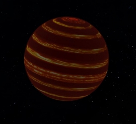
Image: Using high-precision brightness measurements from NASA’s TESS space telescope, astronomers found that the nearby brown dwarf Luhman 16 B’s atmosphere is dominated by high-speed, global winds akin to Earth’s jet stream system. This global circulation determines how clouds are distributed in the brown dwarf’s atmosphere, giving it a striped appearance. Credit: Daniel Apai.

The lighter zones shown above are thought to be thin cloud decks illuminated by light from the hot interior, while the darker zones are where thicker cloud decks block interior light. The wind speeds are highest at the equator, dropping at the higher latitudes. The global wind pattern is lost at the poles, which are a region of enormous local storms, as on Jupiter. Most of Luhman 16 B, then, is dominated by global wind patterns rather than localized storms.

Something of a surprise to the team (the paper refers to the development as ‘a stunning feature’) is the changeable, non-periodic nature of the Luhman 16 light curve. Here’s how the authors describe this fact:

…we identify four properties that are shared between the visual lightcurve of this object and the infrared lightcurves of other objects: 1) The lightcurves remain variable over long periods (years); 2) The lightcurve shape evolves, yet it displays characteristic period, which is likely the rotational period of the object (as found in Apai et al. 2017); 3) In spite of the rapid evolution of the lightcurve, the amplitudes over rotational time-scales remain similar and characteristic to the object; 4) The lightcurves tend to be symmetric in the sense of similar amount of positive–negative features, in contrast to, for example, a situation in which a single positive feature appears periodically on an otherwise flat lightcurve, which would indicate a single bright spot in the atmosphere.

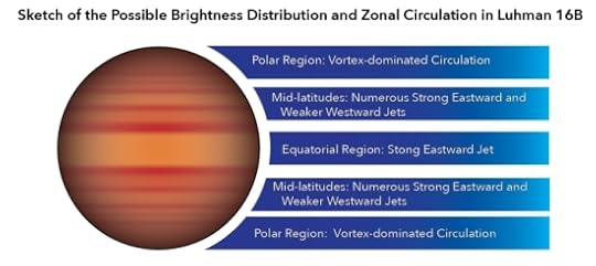
Image: This is Figure 16 from the paper. Caption: Sketch of the possible appearance of Luhman 16B, based on the emerging evidence. Zonal circulation models and comparison to Jupiter suggests that low-latitude regions are dominated by the fastest jets, and that wind speeds at mid-latitude are significantly lower. Circulation at the polar regions is likely to be vortex- and not jet-dominated. Cloud cover is likely to be correlated with the atmospheric circulation. Credit: Apai et al.

All this is drawn from TESS lightcurves of Luhman 16 AB covering 22 days and 100 rotations of the binary, allowing the researchers to conclude that both the brown dwarfs in this system show zonal circulation and fit the Jupiter model. It seems apparent that brown dwarfs can serve as more massive analogs of giant exoplanets and could thus help us develop techniques of atmospheric analysis that can be deployed even further from the Solar System. Says Apai:

“No telescope is large enough to provide detailed images of planets or brown dwarfs. But by measuring how the brightness of these rotating objects changes over time, it is possible to create crude maps of their atmospheres – a technique that, in the future, could also be used to map Earthlike planets in other solar systems that might otherwise be hard to see… Our study provides a template for future studies of similar objects on how to explore – and even map – the atmospheres of brown dwarfs and giant extrasolar planets without the need for telescopes powerful enough to resolve them visually.”

The paper is Apai et al. “TESS Observations of the Luhman 16 AB Brown Dwarf System: Rotational Periods, Lightcurve Evolution, and Zonal Circulation,” Astrophysical Journal Vol. 906, No. 1 (7 January 2021). Abstract / preprint.

Juno at Jupiter: Extended Mission Flybys of Galilean Moons

The news that NASA will extend the InSight mission on Mars for two years, taking it through December of 2022, is not surprising, given the data trove the mission team has collected through operation of the mission seismometer. A live asset on Mars also deepens our knowledge of the planet’s atmosphere and magnetic field, all reasons enough for pushing for another two years. But the extension of the Juno mission to Jupiter deserves more attention than it’s getting, given that Juno’s remit will be expanded deep into the Jovian system.

Image: NASA has extended both the Juno mission at Jupiter through September 2025 and the InSight mission at Mars through December 2022. Credit: NASA/JPL-Caltech.

For those of us fascinated with the outer system, this is good news indeed. I’m looking over two documents, the first being a presentation based on a report submitted to NASA’ Outer Planets Assessment Group (thanks to Ashley Baldwin for passing this along). The OPAG document was produced by Scott Bolton (Southwest Research Institute); it gives the overview of what a mission extension could look like. Also on my desk this morning is the text of the 2020 Planetary Missions Senior Review (PMSR), outlining a set of three mission scenarios. The context of both analyses is the success of the mission in studying Jupiter’s interior structure, magnetic field and magnetosphere, not to mention the examination of its atmospheric dynamics, seen in such roiling imagery as that depicted with stunning complexity in many of the JunoCam images.

Launched in 2011 and operational at Jupiter since 2016, Juno’s prime missions were to have ended in July of this year, with the spacecraft having completed 34 polar orbits, each of 53 day duration. The OPAG report refers to the subsequent extended mission as “a full Jovian system explorer with close flybys of satellites and rings.” The extended mission is to last through September, 2025, with observations of the planet’s ring system, its large moons, and a series of targeted observations and close flybys of Ganymede, Europa and Io.

That last clause really got my attention, as I hadn’t seen it coming. Juno is in an elliptical orbit with a 53-day period whose perijove migrates northward. This bit from the Senior Review reveals in depth the interactions between the various mission scenarios and satellite flybys. The three scenarios mentioned offer alternatives given varying science and budget considerations:

The proposed Juno extended mission (EM) would take advantage of the natural northward progression of the periapsis of the spacecraft’s orbit and the consequent lowering of spacecraft altitudes over Jupiter’s high northern latitudes. The EM would run until the end of the mission, with an expected duration of approximately four years. Under the High and Medium Scenarios, propulsive maneuvers would be utilized not only to target Jupiter-crossing longitude and perijove altitude, as during the prime mission, but also to target close flybys of Ganymede, Europa, and Io. The flyby maneuvers would act to shorten the spacecraft orbital period, yielding more close passes of Jupiter within a given time interval, and increase the rate of northward movement of spacecraft perijove. Under the Low scenario for EM operation, the satellite gravity assists and close satellite flybys would not be attempted.

So mission scientists have a number of options to work with. The extended mission investigates the northern hemisphere and probes the region above Jupiter’s polar cap aurora. The northern adjustment in Juno’s orbit is what makes the satellite flybys possible and enables as well close analysis of its ring structures. The Juno team can look forward to 3D mapping of Jupiter’s polar cyclones and studies of the planet’s unusual dilute core, the latter an earlier Juno discovery revealing a core consisting of both rocky material and ice as well as hydrogen and helium.

Both Europa Clipper and the European Space Agency’s JUICE mission (Jupiter Icy Moons Explorer) should benefit from Juno data on the radiation environment they will operate within. At Europa, Juno will continue the search for possible plume activity while examining the ice shell and mapping surface features, while studies of Io’s magma, polar volcanoes and interactions with Jupiter’s magnetosphere will be enabled by its encounters there. At Ganymede, magnetospheric interactions and surface composition data should be produced in abundance.

In the OPAG presentation, most of the Juno flybys will be at Io, with 11 possible between mid-2022 and 2025. Two encounters are planned for Ganymede (and recall that JUICE is scheduled to orbit the huge moon), and three encounters are feasible for Europa. The actual number of flybys will, according to the Senior Review, depend upon budget choices. In that document, I find this overview of Juno’s satellite flybys:

The orbit of Juno in the EM [extended mission] would take the spacecraft through the Io and Europa plasma tori and in close proximity to Io, Europa and Ganymede. Maps of Ganymede’s surface composition would allow studies to understand the importance of radiolytic processes in surface weathering, identify changes since Voyager and Galileo, and search for new craters. Juno’s Microwave Radiometer (MWR) is particularly sensitive to the upper 10 km of Europa’s ice shell. Studies at wavelengths complementing expected results from Europa Clipper’s radar would identify regions of thick and thin ice and search for regions where shallow subsurface liquid may exist. Juno’s visible and low-light cameras would search Europa for active plumes and changes in color/albedo that may reveal eruption regions since Galileo. The fields and particles experiments would look for evidence of recent activity. Finally, the Juno EM would include a flyby of Io and search for evidence of a magma ocean.

What an interesting development Juno’s extended mission turns out to be! Continuing science operations with existing equipment far undercuts the cost of new missions while extending long-duration datasets and, in the case of Juno, enabling a set of exciting new targets. We have the option here of a series of Galilean moon flybys that were never in Juno’s original mission, observations that could inform later choices made for Europa Clipper and JUICE. All told, Juno’s unanticipated extended mission is a heartening contribution to outer system science.

Hayabusa2: Multiple Paths for Analyzing an Asteroid

Ryugu is classified as a carbonaceous, or C-type asteroid, a class of objects thought to incorporate water-bearing minerals and organic compounds. Carbonaceous chondrites, the dark carbon-bearing meteorites found on Earth, are thought to originate in such asteroids, but it has been difficult if not impossible to determine the source of most individual meteorites.

Hence the significance of the Hayabusa2 mission. JAXA’s successful foray to Ryugu represents the first time we’ve been able to examine a sample of a C-type asteroid through direct collection at the site. Ralph Milliken is a planetary scientist at Brown University, where NASA maintains its Reflectance Experiment Laboratory (RELAB). The laboratory expects samples collected at Ryugu to arrive in short order. Milliken is interested in the history of water in the object:

“One of the things we’re trying to understand is the distribution of water in the early solar system, and how that water may have been delivered to Earth. Water-bearing asteroids are thought to have played a role in that, so by studying Ryugu up close and returning samples from it, we can better understand the abundance and history of water-bearing minerals on these kinds of asteroids.”

Milliken is also one of many co-authors on a new paper in Nature Astronomy looking at the thermal history of subsurface materials exposed on Ryugu. The paper examines data the spacecraft collected during its operations there, which can now be compared to the sample collection. We learn that the asteroid may not be as water-rich as originally thought, leading to various scenarios about how it might have lost its water. High on the list of possibilities is that this ‘rubble pile’ asteroid — essentially loose rock maintaining its shape because of gravity — dried after a collision or other disruption and subsequent reformation.

Image: Japan’s Hayabusa2 spacecraft snapped pictures of the asteroid Ryugu while flying alongside it two years ago. The spacecraft later returned rock samples from the asteroid to Earth. Credit: JAXA.

Bear in mind how Hayabusa2 proceeded with its sampling at Ryugu. During the 2019 rendezvous, the spacecraft fired a projectile into the asteroid’s surface that exposed the subsurface rock examined here. A near-infrared spectrometer was used to compare the water content of the surface with the material below, showing the two to be similar in water content. The authors see that as a clue that Ryugu’s parent body dried out, rather than the surface of Ryugu being dried out by the Sun, perhaps in a close solar pass earlier in its history.

In other words, heating by the Sun in one or more close solar passes would be likely to occur at the surface, without penetrating deep into the asteroid. What Hayabusa2’s spectrometer shows is that surface and sub-surface are both comparatively dry, which is an indication that it was the parent body of Ryugu, rather than an event happening to Ryugu itself, that produced this result.

Ahead for the Ryugu analysis is the need to study the size of the particles excavated from below the surface, which could play a role in how the spectrometer measurements are interpreted.

“The excavated material may have had a smaller grain size than what’s on the surface,” says Takahiro Hiroi, a senior research associate at Brown and another study co-author. “That grain size effect could make it appear darker and redder than its coarser counterpart on the surface. It’s hard to rule out that grain-size effect with remote sensing.”

The beauty of the successful sample return is that hypotheses about Ryugu’s past can now be evaluated through comparison of the remote sensing data and actual laboratory work. These are exciting times indeed for the scientists studying the extensive collection of asteroid debris Hayabusa 2 brought back. We can expect significant papers on all this in 2021.

The paper is Kitazato et al., “Thermally altered subsurface material of asteroid (162173) Ryugu,” Nature Astronomy 4 January 2021 (abstract).

The Red Dwarf Habitable Zone Dilemma

Henry Cordova, whose recent critique of traditional SETI kicked off a lengthy discussion in these pages, has been mulling over issues of habitability in the galaxy’s vast population of red dwarf stars. While we’ve focused on the questions raised by stellar flare activity and the climate challenges of tidal lock, the narrow band of habitability among the fainter M-dwarfs poses its own problems. How big a factor is a narrow circumstellar habitable zone? Henry comes by his interest in these matters by way of US Navy training in both astronomy and mathematics. A retired geographer and map maker now living in southeastern Florida, he’s keeping up with exoplanetary issues as an active amateur astronomer and collector of star atlases.

by Henry Cordova

I am curious as to how the width of a star’s habitable zone varies with respect to its luminosity.

It would not be unreasonable to assume that the surface temperature of a planet is directly related to the radiant flux of its star. Furthermore, it seems reasonable that the range of surface temperatures in which water can be a liquid on at least part of a planet’s surface is directly related to the stellar flux at its orbital distance. There may be many other factors involved, such as the properties of the planet’s atmosphere, its rotational characteristics, orbital elements and the variability and spectrum of its parent star; but let us ignore them for the moment and simply consider the geometrical parameters involved.

All else being equal, the radiant flux received by the planet must then be directly proportional to the luminosity of the star, and inversely proportional to the square of the planet’s distance from it. In other words, if one star is a hundred times more luminous than another, a planet orbiting the fainter star must be ten times closer to its primary in order to receive the same flux. The same reasoning can be applied to both the inner and outer edges of the star’s habitable zone. Regardless of how we define the HZ, it will become much narrower as the luminosity of the primary decreases. And the narrower an HZ is, the less likely there is a planet there.

Consider our own Sun’s habitable zone. Although there is some controversy about its dimensions, let us for the purposes of this argument say that it is limited by the orbits of Mars and Venus.The two planets have semi-major orbital axes of roughly 1.5 and 0.7 AU, respectively. These two figures mark the limits of Sol’s HZ, and their difference gives an HZ width of 0.8 AU, plenty of room to squeeze Earth in.

If our Sun were a hundred times less luminous, the HZ boundaries would be at 0.15 and 0.07 AU, which translates to an HZ width of only 0.08 AU! Clearly, the HZs of faint stars can be very narrow. The chances of a planet forming there, or migrating in, are substantially reduced.

Astronomers have detected planets in the HZs of some red dwarfs, but I feel this is due primarily to selection effects. Many of our planet detection techniques are very sensitive to big planets orbiting small stars in close, highly elliptical orbits, circumstances which are not conducive to life and yielding statistics that may give us a distorted idea of how solar systems form. Because of these considerations, red dwarfs may not be good candidates for life, even if we disregard other problems such as flares and tidal locking. It is true that these stars are often old, stable for long periods of time and by far the most common type of star, but I think we’re better off looking at brighter main sequence stars, such as spectral classes K, G or even F.

Several recent papers have pointed out that albedo effects on the planets of red dwarf stars may significantly expand the sizes of their habitable zones. See Joshi and Haberle, “Suppression of the water ice and snow albedo feedback on planets orbiting red dwarf stars and the subsequent widening of the habitable zone,” Astrobiology Vol. 12, No. 1 (23 Jan 2012); here’s the abstract. For Centauri Dreams‘ discussion on this, see M-Dwarfs: A New and Wider Habitable Zone.

These monographs suggest that on worlds with significant snow and ice cover, the effective albedo is much lower than snow and ice on Earth because frozen water absorbs more radiant heat at the red and infrared wavelengths emitted by red dwarfs than it does in the visual part of the spectrum as in Sol’s case. This effect would certainly extend the size of the habitable zone, but that would be dwarfed (no pun intended) by the much greater inverse square law effect (several orders of magnitude) of the much lower M-dwarf stellar luminosity.

Of the 53 known systems (66 stars) within 5 parsecs (16.3 ly) of the Sun, there are 48 red dwarfs (spectral class M) ranging from absolute magnitude 8.09 to 16.20 (an enormous range of luminosities!), and only 2 of them brighter than absolute magnitude 10.0. Absolute magnitude is the intrinsic brightness, how bright the star would appear if it were exactly 10 pc distant.

Keep in mind that magnitudes are exponential: A 5th magnitude star is 100 times brighter than one of 10th magnitude. Or alternatively, each magnitude is 2.512 times brighter than the next. The Sun’s absolute magnitude is 4.84, Barnard’s star, 13.23. Proxima Centauri is absolute magnitude 15.56. Although our own Sun is considered to be in the mid-range of stellar luminosities, it is still much brighter than most other stars. Red dwarfs may be very numerous, but they are very, very faint. All together, they don’t provide much habitable space.